Category: DevOps and Open Technologies

Editorial Calendar for February 2016

  • How do we Bring APIs Into Decentralized Web3?

    How do we Bring APIs Into Decentralized Web3?

    Blockchain-based applications are growing in popularity and underscore the decentralized Web3 movement. Simultaneously, web APIs are helping port data and reusable functionality across application types and are driving microservices development practices. So, how do we bring these two paradigms together?

    There are many cases where a blockchain-based smart contract may require data updates that only a web API request can fulfill. For example, perhaps the smart contract needs to access the latest price of a given stock ticker. Or, perhaps on-chain activities are contingent on the weather at a particular time. The ubiquity of APIs means there are thousands of helpful features available for the task at hand. Yet, integrating them into Web3 applications is tricky.

    Interestingly, the API3 Alliance is making strides to introduce an industry-standard solution to bring APIs to Web3 applications. API3 provides a vendor-neutral standard gateway to apply on top of existing APIs that helps them appeal to decentralized apps. The vendor-neutral API Alliance already consists of many APIs across various verticals and appears to be gaining more traction.

    I recently met with API3’s co-founder, Heikki Vänttinen, to learn more about the challenges of introducing traditional web APIs into blockchain development. According to Vänttinen, whereas previous solutions relied on a third-party middleware or ‘oracle,’ the best way to incorporate an API request and response system into smart contracts is through a node operated by the API provider themselves. Such a system could help blockchain-based applications leverage myriad software-as-a-service solutions, essentially uniting the two worlds.

    The State of APIs in Web3

    The number of APIs is growing exponentially. As companies reinvent themselves with digital transformation, APIs have become the glue for interconnecting the applications we use on a daily basis. When it comes to APIs, there are a growing number of potential use cases for blockchain—the technology is not just relegated to cryptocurrency; rather, it can power a number of scenarios that require smart ledgers.

    Since APIs drive much of the functionality in modern software development, it makes sense that they may be useful in decentralized app development. For example, a blockchain-based decentralized finance (DeFi) app that handles lending and borrowing may want to call an API to collect raw data for a liquidation price, says Vänttinen. Or, a smart contract may wish to acquire the cost of an asset as a conditionality for making a purchase. Hooking into public APIs to check local weather or flight arrival information could affect how smart contracts respond.

    There are many use cases for incorporating APIs into a distributed ledger system. However, “blockchain applications are not able to call APIs natively,” Vänttinen explained. The incompatibility is due to the nature of blockchain technology, said Vänttinen, as it requires consensus from multiple parties to maintain the smart contracts. For this reason, blockchain applications require a middleware piece to connect a blockchain node to an API, relaying data responses from outside of the chain.

    Incorporating APIs Into Blockchain

    As Vänttinen described, previous attempts to connect APIs to Web3 architectures have revolved around a third-party middleware node. Yet, externalizing integration responsibility in this way creates a centralized point of failure, which defeats the purpose of a decentralized environment altogether.

    Instead of relying on such a dependency, Vänttinen advocates for a “first-party oracle approach,” in which API providers operate a layer in front of their APIs. This enables a request-response mechanism for smart contracts, allowing blockchain applications to initiate API requests from on-chain and incorporate the responses into the contracts. This method retains immutability and trustlessness, which is inherent to the distributed ledger.

    One solution enabling such an architecture is Airnode, a Web3 middleware that connects any web API directly to any blockchain application. Companies that have adopted Airnode make up the API3 Alliance, which is “a collective of API providers who have signed up to enable this first-party use of their API for Web3 applications,” said Vänttinen. “Adopting Airnode is a pledge from API companies to make their API blockchain-compatible.”

    The API3 Alliance is one significant initiative aiming to extend the capabilities of smart contracts and blockchain applications. This could enable such environments to call an API to send a text message or email, or grab sports scores, collect maps data and so on. Thus far, participating APIs in the API3 Alliance come from sectors such as agriculture, biotechnology, communications, open banking, insurance, supply chain management and many others. The initiative also accepts applications from API providers that want to join the marketplace.

    Benefits of a Common Web3 Integration Layer

    So, what are the benefits of embracing an industry-standard middleware for web-API-to-blockchain connectivity? Well, according to Vänttinen, it is the best way to enable complex off-chain computation. Enacting intricate computing on the chain is quite resource-intensive, resulting in high transaction fees. By extending particularly complicated calculations externally, blockchain applications could reduce operational overhead. “The industry is long overdue for connection between the real world and blockchain,” said Vänttinen. (By real-world, I assumed he meant other architectural styles that pre-date blockchain.)

    Having a standard implementation could also reduce the development burden for the API provider to support nuanced technologies. Whereas other solutions would require someone in-house to operate blockchain nodes, Airnode is more of a plug-and-play API gateway that could be deployed on AWS as a Lambda function, Vänttinen said. This usability makes it easy for API-based services to appeal to Web3 applications, thus quickly opening a new potential growth segment.

    Of course, Vänttinen admitted, the concept of syncing with off-chain processes is still at a very early stage. There are competing philosophies about how to address it on the market, and some foundational issues have not yet been resolved. For example, most efforts have focused on Read operations to acquire raw data. The next step will be having the middleware ‘oracle’ incorporate off-chain Write capabilities, too. Furthermore, more PubSub-like formats will be important to enable event listeners capable of reactive qualities.

    Final Thoughts

    The Web3 trend is bringing more decentralized, blockchain-based applications to fruition. But, such applications can’t operate in a closed-off world. To experience the full breadth of digital possibilities, they’ll likely need to figure out how to incorporate off-chain computations and mesh with alternative communication software libraries. Naturally, this will require integrations with web APIs, which have become an important method of cloud-based communication.

    The API3 Alliance is “here to propose a solution to the API connectivity problem for Web3,” said Vänttinen. “When a data provider is blockchain-compatible, you can apply the reputation of the data provider in this decentralized data feed … The importance of this becomes more clear when you talk about connecting off-chain services and microservices with smart contracts.”

    Airnode and the surrounding API3 Alliance is one initiative spearheading the connection of APIs and smart contracts. But, this is just one method in a maturing field. What do you think about bridging the two paradigms? Comment on your experience below!

  • HashiCorp Previews Updates to Consul Service Mesh

    HashiCorp Previews Updates to Consul Service Mesh

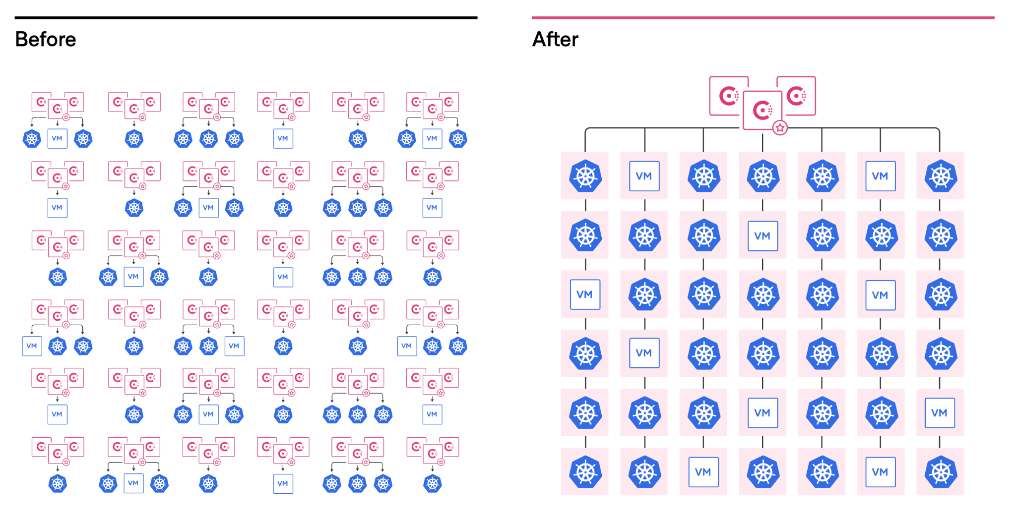
    During an online HashiConf Global conference, HashiCorp today made available a beta of an update to its open source Consul service mesh for virtual machines and Kubernetes clusters that makes it possible for multiple administrators to share the same instance of a multitenant service mesh.

    Version 1.11 of Consul will also add support for a command line interface (CLI) for Kubernetes that will provide an alternative to Helm charts for installing Consul on those clusters.

    Raymond Austin, director of product marketing for HashiCorp, said it’s become apparent that there is a need for a higher level of abstraction for managing application programming interfaces (APIs) that is easy to deploy across both legacy IT environments based on virtual machines and cloud-native environments based on Kubernetes clusters.

    Of course, in many cases, those Kubernetes clusters are deployed on top of virtual machines. However, there are also now more instances of Kubernetes being deployed on bare metal platforms at, for example, the network edge.

    As IT environments become more complex, a service mesh makes it simpler to discover, access and secure APIs that are now rapidly proliferating across the enterprise. That transition requires a more dynamic approach to not only managing APIs but also the network services those APIs depend on, added Austin.

    HashiCorp is betting that many IT organizations will prefer to rely on a lightweight open source platform supported by a single vendor rather than relying on more complex open source service mesh offerings being developed under the auspices of a consortium.

    It’s still not quite clear who within an IT organization is assuming responsibility for deploying a service mesh. Most often, it’s a development team that makes the initial decision. However, as IT operations teams become more aware that service meshes represent a capability that needs to be horizontally made available across multiple applications, it may be only a matter of time before some organizations decide to standardize on a single service mesh to reduce operational overhead, noted Austin.

    Service meshes will also play a critical role in simplifying management of networking and security services at a higher level of abstraction within a larger DevOps workflow.

    It’s still early days as far as service mesh adoption in the enterprise is concerned, but there are already a large number of service mesh options. In fact, there may never be a single dominant service mesh platform. Interoperability standards still need to be ratified that enable organizations that have standardized on different service meshes to apply policies to microservices spanning hybrid cloud computing environments.

    Of course, not every IT organization requires a service mesh yet, either. Many IT teams can still get by using a traditional proxy server or an API gateway until the number of microservices-based applications deployed starts to achieve critical mass. One way or another, however, the more APIs there are to manage, the more inevitable it becomes that an IT team will deploy a service mesh.

  • Pulumi Adds Registry to Share Secure IaC Code

    Pulumi Adds Registry to Share Secure IaC Code

    Pulumi this week added a public registry to its portfolio that makes it easier to discover packages that have been created using its tools to manage infrastructure-as-code (IaC).

    Joe Duffy, Pulumi CEO, said the Pulumi Registry will make it simpler for DevOps teams to share and reuse IaC tools that have been vetted versus always requiring each development team to write new code each time they want to programmatically provision infrastructure. Pulumi Packages provide modern cloud reference architectures in the form of software development kits (SDKs), code samples and how-to guides.

    One of the primary reasons that security has become a major cloud issue is that developers often misconfigure infrastructure. The registry provides a way to reduce those configuration errors by making it easier for developers to reuse code written in TypeScript/JavaScript, Python, Go and .NET that they have stored in repositories such as npm.

    In addition to the major cloud service providers, there are also Pulumi Provider Packages for Auth0, CloudFlare, Confluent Cloud, Datadog, DigitalOcean, Docker, GitHub, Kong, MinIO, MongoDB Atlas, PagerDuty, Snowflake, Spot by NetApp and others.

    There are also Pulumi Component Packages for deploying container applications on instances of Kubernetes and other related platforms in addition to deploying applications on serverless computing frameworks.

    Duffy said in addition to providing a “golden image” of their configurations the registry reduces the overall level of friction that often exists between developers, IT operations teams and cybersecurity professionals.

    The latest Pulumi offering is part of an ongoing effort to democratize cloud computing in a way that is repeatable and reliable, noted Duffy. Pulumi, for example, just added support for a set of AWS Cloud Control application programming interfaces (APIs) that reduce the number of APIs that developers would otherwise have to master. The more APIs there are, the more likely it is a developer will make a mistake.

    IT teams should expect that other cloud service providers will similarly streamline the APIs they present developers as part of an effort to make their services both more accessible and secure. In the meantime, frameworks provided by Pulumi provide a means to invoke those lower-level APIs at a higher level of abstraction for both developers and internal IT operations teams alike.

    It’s not clear today how many developers routinely employ IaC tools, but as the number of workloads deployed in the cloud steadily increases, so too does the percentage of developers that employ these tools. While that shift represents a major boon in productivity for developers, it brings with it additional security risks that many organizations fail to appreciate until it’s too late.

    The only way to really solve that issue is for organizations to adopt DevSecOps best practices that require a level of collaboration between DevOps and security teams that is still relatively rare. However, as the tooling provided continues to improve, the technical challenges associated with achieving that goal continue to decline. The next big issue, as always, is bringing together all the diverse cultures within an IT organization to actually implement those tools and define a set of best practices that work for all concerned.

  • Splunk Donates eBPF Telemetry Data Collector to CNCF

    Splunk Donates eBPF Telemetry Data Collector to CNCF

    Splunk Inc. announced during the KubeCon + CloudNativeCon North America conference that it donated a data collector to the OpenTelemetry project run by the Cloud Native Computing Foundation (CNCF).

    Splunk’s data collector runs as a sandbox-level program at the kernel of a Linux operating system and takes advantage of extended Berkeley Packet Filter (eBPF) technology to make it simpler to collect networking telemetry.

    The OpenTelemetry initiative itself spans a range of open source tools, application programming interfaces (APIs) and software development kits (SDKs) that are used to instrument applications. Previously, Splunk contributed the SignalFx Smart Agent and Smart Gateway to the OpenTelemetry project along with more than 64,000 code contributions.

    Morgan McLean, a director of product management for Splunk, said that while OpenTelemetry is officially in beta, some elements of the project are more mature than others. For example, tools for capturing metrics and traces are already being employed, while another set of tools for capturing log data will be ready sometime next year, he said.

    The data collector contributed by Splunk is among the first that operate at the kernel level to collect data, added McLean. That approach makes it possible for some types of data to be captured by default rather than requiring developers to always instrument their applications using agents to enable an observability platform. It will also contribute toward the eventual convergence of network operations and DevOps processes.

    Going forward, DevOps teams should expect to employ a mix of open source data collectors that operate at both the eBPF and application level, said McLean. The eventual goal is to instrument every application by default by making it much simpler to collect data. Today, most DevOps teams are employing a mix of proprietary and open source agent software to collect data that then must be deployed and then integrated with all the applications they build. Given the cost and level of effort required, the percentage of applications that are actually instrumented is, not surprisingly, fairly low.

    However, as agent software becomes more readily accessible, the percentage of applications that are instrumented should increase considerably in the years ahead. For DevOps teams that depend on that data to optimize application performance, that capability should prove to be a boon for improving overall observability in IT environments.

    Observability, in one form or another, has always been a core tenet of any DevOps best practice. Initially, DevOps teams focused on continuous monitoring as the most effective way to proactively manage application environments. However, it can still take days, sometimes weeks, to discover the root cause of an issue.

    Monitoring focuses on predefined metrics to identify when a specific platform or application is performing within expectations. The metrics tracked generally focus on, for example, resource utilization. Observability platforms combine metrics, logs and traces—a specialized form of logging—to instrument applications in a way that makes it simpler to troubleshoot issues without relying on a limited set of predefined metrics focused on a specific process or function.

    Those observability platforms then make it possible to correlate events so that it is easier to identify anomalous behavior indicative of an issue’s root cause. Armed with these insights, it becomes a lot simpler for IT teams to resolve issues faster.

    It’s unclear when OpenTelemetry tools will become more widely employed, but as more tools for collecting data become available, the impact on DevOps will be nothing short of profound.

  • CNCF Adopts Meshery to Advance Service Mesh Management

    CNCF Adopts Meshery to Advance Service Mesh Management

    The Cloud Native Computing Foundation (CNCF) announced this week during the ServiceMeshCon/KubeCon + CloudNativeCon conference that Meshery, a service mesh management plane created by Layer5, has become a sandbox-level project.

    In addition, Layer5 has also donated Service Mesh Performance (SMP), a set of tools for measuring the efficiency of a service mesh, to the CNCF. SMP provides an open source framework to define standardized benchmarking practices, performance test configurations and measurements as part of an effort to create a MeshMark index for rating a service mesh. A set of service mesh performance methodologies will also be published by the IEEE later this month, developed in collaboration with engineers from Layer5, Intel, Red Hat and HashiCorp.

    Layer5 CEO Lee Calcote said the goal is to make it simpler for IT teams to determine which service mesh to employ based on their specific use case requirements.

    Several service mesh platforms are starting to gain traction as a means to both manage application programming interfaces (APIs) and provide a layer of abstraction between lower-level networking and security APIs that makes those services more programmatically accessible to developers.

    Meshery itself is an implementation of SMP and the conformance tool created for the Service Mesh Interface (SMI), a separate CNCF project to promote interoperability between service meshes. Meshery is based on a set of microservices that are designed to make the platform easily extensible.

    That approach makes it possible to manage multiple instances of service meshes that might be deployed on virtual machines as well as Kubernetes clusters using a range of management tools that are part of the Meshery project.

    Meshery supports AWS App Mesh, Citrix Service Mesh, HashiCorp Consul, Istio, Kuma, Linkerd, Network Service Mesh, NGINX Service Mesh, Open Service Mesh and Traefik Mesh. Meshery also provides IT teams with more than 60+ best practices in the form of templates that can be used to deploy a service mesh.

    It’s still early days as far as adoption of service mesh in the enterprise is concerned. Most IT teams still rely on either proxy software or a gateway to manage APIs. However, as the number of APIs that need to be managed steadily increases, it won’t be long before many IT teams start to at least evaluate a service mesh.

    In the longer term, the impact those service meshes are likely to have on the management of IT could be profound. It is becoming apparent that a service mesh also provides a higher level of abstraction for invoking networking and security services. In fact, the service mesh may wind up playing a key role in driving the convergence of network and security operations with DevOps best practices.

    In the meantime, IT teams will need to decide to what degree they may want to standardize on a single service mesh versus letting individual teams implement their own preferred platform that could one day be centrally managed via Mashery. One way or another, the way APIs are managed and invoked will soon fundamentally change forever.

  • New Relic I/O Aims to Simplify Instrumentation

    New Relic I/O Aims to Simplify Instrumentation

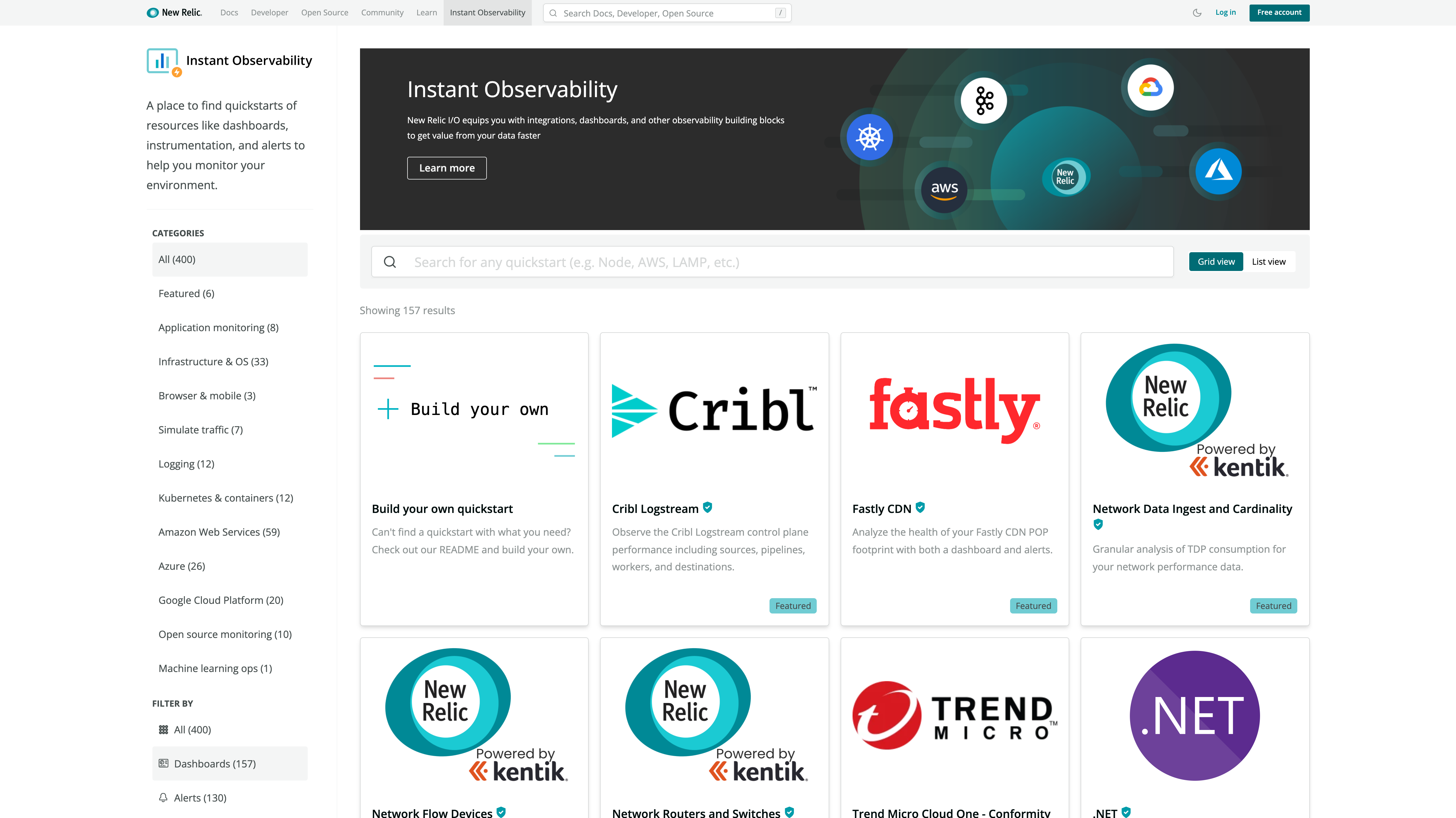
    New Relic today at the KubeCon + CloudNativeCon North America conference launched a New Relic Instant Observability (I/O) initiative through which it is making available open source tools to simplify application instrumentation.

    Marck Robinson, senior vice president for engineering at New Relic, said the catalog of tools will help DevOps teams instrument a much wider range of applications. New Relic will make those tools available as part of the free tier of its observability platform delivered via the cloud. DevOps teams will be able to use more than 400 pre-configured quickstarts to both instrument applications and create dashboards, Robinson said.

    New Relic itself is contributing quickstarts for cloud services, open source tools and platforms such as Kubernetes, Istio and Cassandra. Third-party vendors that have already contributed to the catalog include Cribl, Fastly, Gigamon, Kentik, Lacework and Trend Micro. Each contribution is being vetted by New Relic as part of an effort to foster the development of a larger open source observability ecosystem, noted Robinson.

    Robinson said overall, New Relic is trying to make it easier for DevOps teams to close an instrumentation gap that is impeding IT organizations from moving beyond monitoring to embrace true observability of their IT environments. The recent New Relic 2021 Observability Forecast report notes only a quarter of respondents (26%) have a mature observability practice, with the most commonly cited barriers to observability being a lack of resources (38%) and skills gaps (29%).

    As a result, DevOps teams often encounter a last-mile observability challenge when it comes to both instrumenting applications and then building their dashboards, said Robinson.

    As part of a larger effort to make it easier to instrument applications, New Relic has open sourced agent software, standardized on the OpenTelemetry tools being advanced under the auspices of the Cloud Native Computing Foundation (CNCF) and contributed the Pixie observability platform for Kubernetes environments to the CNCF.

    Observability in one some or another has always been a core tenet of any DevOps best practice. Initially, DevOps teams focused on continuous monitoring as the most effective way to proactively manage application environments. However, it can still take days, sometimes weeks, to discover the root cause of an issue. However, observability platforms are emerging that correlate events in a way that makes it easier for analytics tools to identify anomalous behavior indicative of a root cause of an IT issue. Armed with these insights, it becomes a lot simpler for IT teams to resolve issues faster.

    In contrast, monitoring focuses on predefined metrics to identify when a specific platform or application is performing within expectations. The metrics tracked generally focus on, for example, resource utilization. Observability, on the other hand, combines metrics, logs and traces—a specialized form of logging—to instrument applications in a way that makes it simpler to troubleshot issues without having to rely solely on a limited set of metrics that have been pre-defined to monitor a specific process.

    With the rise of microservices-based applications, the shift to the cloud and more end users than ever working remotely, the need for observability has never been more critical. The issue now is finding a way to make it much simpler to achieve.

  • LF Networking (LFN) Adds to Open Source Portfolio

    LF Networking (LFN) Adds to Open Source Portfolio

    At the online Open Networking & Edge Summit + Kubernetes on Edge Day event LF Networking (LFN), an arm of the Linux Foundation focused on networking, today added several projects that promise to make it simpler to programmatically manage networking services based on open source software.

    Walmart is contributing a L3AF project for managing network applications that make use of an extended Berkeley Packet Filter (eBPF) capability that allows applications to run in a sandbox at the microkernel level of an operating system. Intel and Aarna Networks, meanwhile, are donating the seed code from an EMCO project that provides a universal control plane to securely connect and deploy workloads across distributed computing environments that span everything from the edge to the cloud.

    Arpit Joshipura, general manager for networking, edge and internet of things (IoT) for the Linux Foundation, said the L3AF project adds a control plane for managing those applications to the LFN portfolio that addresses load balancing, rate limiting, traffic mirroring, flow exporter, packet manipulation, performance tuning and other management tasks. Earlier this year, the Linux Foundation set up a separate eBPF Foundation to further advance development and adoption of eBPF across multiple operating systems.

    At the same time, LFN also revealed today that Project Alvarium, a tool for measuring how well data is being delivered to devices that was originally created by Dell, and eKuiper, an existing open source lightweight IoT data analytics and streaming platform, are now part of the LF EDGE portfolio of projects.

    Finally, an open source mobile edge computing project, dubbed Edge Gallery, that was originally created by Huawei has been contributed to the Linux Foundation.

    Joshipura said the LFN continues to gain momentum as more vendors contribute core technologies that, ultimately, don’t provide them with enough differentiated value to continue to develop on their own. The LFN today also revealed that VMware and F5 Networks have joined the LF EDGE consortium as premier members, while mimik and Veena, Inc. have become general members of LFN and the Eclipse Foundation has become an associate member.

    The LFN also provides a mechanism that promotes adoption of those technologies more widely than any one vendor can achieve on its own. The total cost of delivering next-generation edge computing platforms based on wireless 5G networks will also be sharply reduced as LFN projects continue to mature, said Joshipura.

    In general, the rate at which various LFN projects are updated continues to accelerate, said Joshipura. The Akraino project for creating blueprints for edge computing platforms recently delivered its fifth update to address use cases involving smart cities, cloud-native multi-tenant environments and vehicular networks. An EdgeX Foundry project for IoT platforms, meanwhile, recently revamped its application programming interfaces (APIs) to make them more secure and enable more message-based communications. The Home Edge project will also soon issue a Drewberries update that will address code stabilization, scripting, APIs, data synchronization and security.

    It’s now only a matter of time before these LFN projects become more integrated with DevOps workflows as IT teams seek to give developers more programmatic control over network services. The issue now is deciding not so much whether to integrate network operations and DevOps teams but rather determining to what degree those teams will need to fold into each other.

  • Closing the Education Gap for IoT Developers

    Closing the Education Gap for IoT Developers

    The most common thing I hear from developers who are building internet of things (IoT) solutions is: It isn’t easy. And it’s not. Not because of a lack of skill—the developers I interact with are incredibly talented. There’s also no shortage of technologies to choose from for deploying an IoT solution. The challenge often comes down to a gap in available educational materials and learning support when in the development phase.

    We’ve moved from the early stages of the IoT when there was a lot of talk but not a lot of application. Now, we’re coming into the “reality phase” where cheaper, large-scale IoT solutions are feasible. In this phase, developers are tasked with identifying, building and deploying technologies that they’re likely having to figure out as they go. It’s a tall order to expect today’s developers to know the ins and outs of all of the moving pieces required for an IoT solution, including the wireless technologies that help to enable them. 

    While developers are renowned for being effective at independent learning, they still need better access to educational resources and tools when it comes to IoT technologies. This is especially true for newer technologies that you won’t yet find in a textbook or college course. 

    One example of this newer IoT technology is low-power, wide area networks (LPWAN)—specifically using the LoRaWAN standard. It’s an area that I not only expect to become increasingly relevant for IoT developers but also one that can greatly benefit from more robust educational resources. 

    IoT Development Is Relatively New 

    Modern LPWAN technologies have only been around for the past decade, and LoRaWAN became an open standard when the LoRa Alliance was formed in 2015. In the grand scheme of things, that’s pretty new. It’s not a concept that’s widely included in higher education curricula and, although we see more inclusion each year, it can be difficult for developers to find peers who have experience in building with LoRa devices. 

    ABI Research forecasts that by 2026, LoRa will be the leading non-cellular LPWAN technology. This means that over the next five years more and more developers will need to understand the basics of LoRaWAN but may not have foundational knowledge or experience to draw from. 

    From what I’ve seen, that gap can lead to teams biting off more than they can chew. Without enough training or support, developers risk building LoRaWAN deployments that may have inadequate coverage or go over scope or budget or that simply don’t live up to their vision.

    Complexity in Developing With IoT

    The other major reason IoT technologies operating with LoRaWAN need more robust educational support is due to their complexity. Developing an IoT solution requires several different skillsets that well-equipped teams either have to account for in their staffing or—as happens in many cases—rely on a single developer to figure it out and wear many hats.

    There are many aspects to building and deploying a LoRaWAN solution; for instance: Hardware engineering, device stack choice and application fit, gateway deployments and networking coverage, cloud considerations and application development involved for deployment. That’s a lot of moving parts.

    So, if enterprises and IoT vendors are expecting developers to make large-scale IoT deployments a reality, we have to provide the proper resources and training.

    Resources and Communities for LoRa Developers

    As the industry works on ways to better educate developers about LoRa technology, there are some good places to start for developers who want to hit the ground running. Here are some resources where you can learn the basics, build prototypes, get advice from other developers and test and certify solutions. 

    • LoRa Developer Portal—A hub where IoT developers can learn, connect with peers and accelerate their builds with resources like tutorials, dev kits and a free network server. Helpful for every level of expertise, from learning the basics of LoRaWAN to creating a network to rolling out a full-scale commercial solution.
    • LoRa Alliance—A nonprofit association where members collaborate and share experiences working with the LoRaWAN standard. They offers events, webinars, a resource hub and more. 
    • LoRa Basics Station —A GitHub Repository for the open source software that runs on gateways operating with the LoRaWAN standard.
    • AWS IoT Core for LoRaWAN—A guide for AWS IoT developers, spanning coverage development and deployment from connecting gateways to monitoring and logging. 
    • Azure IoT Hub—Guide for connecting the ChirpStack open source network server using LoRaWAN to the Azure IoT Hub.

    I expect higher education institutions to begin further integrating LoRaWAN into their curricula over the next several years, which will help to fill the education gap for the next wave of developers. At the same time, IoT vendors can step up and provide additional support to developers who are learning how to build with technologies like LoRa for the first time. This is critical for the success of large-scale deployments that all of us IoT believers hope to see across enterprise environments, cities, regions and beyond.

  • Microservices Adoption and the Software Supply Chain

    Microservices Adoption and the Software Supply Chain

    Software development is undergoing industrialization, with more and more software rapidly assembled out of components and an emphasis on building automation around software validation and release processes.

    Modern cloud-native software is no longer a monolithic application living in a single repo with the majority of its dependencies self-contained. It is integrated from third-party components provided by vendors, cloud providers and open source software (OSS) components, with as much as 90% of code coming from such dependencies. This allows developers to build applications much faster but makes maintenance much harder as it is no longer entirely under their control. If the third-party vendor makes a change to their API, developers are on the hook to update their applications before they break. 

    Each microservice interacts with hundreds of other microservices and each is built and released independently, making it hard to understand how to coordinate API changes across them. For example, if you want to make an API change to a microservice, what impact will this have on the consumers in the organization? Who will need to coordinate the change? When it was all within the same repository and released all at once, it was much easier to make such changes.

    The Changing Nature of Technical Debt

    What we continue to call technical debt is really the activities that are related to tending to and upgrading our software when third-party components are evolving or have common vulnerabilities and exposures (CVEs) and need to be upgraded.

    These are tedious, repetitive tasks that usually fall to the most experienced engineers as they require technical expertise to do correctly. Such activities can paralyze engineering organizations and are a tremendous burden on engineers; that often leads to burnout. Up to 30% of engineering time is spent on technical debt. The perception that somehow developers were responsible for accruing this technical debt and are doing something wrong that prevents them from keeping up is hugely demoralizing and demotivating. 

    However, if we reframe technical debt as software supply chain management and stop blaming engineering for it, we can make maintenance more predictable and consistent. By taking steps like inventorying third-party components and determining how pervasive they are in the application (frameworks take more effort to maintain than a third-party API that you just call from one part of the application), an organization can arrive at a maintenance estimate. 

    These activities are highly repetitive across organizations, as everyone is integrating some subset of the same third-party components to create business value. This high level of repeatability points us to automation. 

    Specialized Developer Tools for Software Maintenance Don’t Exist

    When developers write code, their hands often lag behind their thoughts. They think much faster than they are able to type the code. You often hear developers finishing a tedious task and complaining, “My fingers hurt.” When their IDE can autocomplete syntax, it helps reduce this lag to minutes.

    When a major framework version is released, developers contemplate the codebase. Maybe they need to change this type to that, reorder some method arguments or change dependencies. The types of changes they need to make are enumerable and must be made almost immediately; again, the ability to implement them lags far behind their recognition of the problem. Often, this type of lag can represent months or years of work when dealing with a large codebase. Accumulate enough of this lag and the codebase can grind to a halt.

    That lag kills the joy in development for most senior developers and leads to burnout. Upgrades/migrations amplify that lag by orders of magnitude.

    However, there are few (if any) tools that focus on helping developers automate these remediations/upgrades/migrations. The IDE’s focus is rightly on helping developers write new code and maintain their own code, but code maintenance needs to be coordinated across multiple places across the codebase, within the same repository or across the repository boundaries. Often, developers have a pattern they want to change in their repository, but the IDE only suggests this as an improvement in their current location (one file). Other times, changes need to be coordinated across repository boundaries if developers want to change APIs and their consumers. That’s why this technology needs to exist outside of the IDE.

    OpenRewrite

    OpenRewrite is an open source project that offers semantic analysis and refactoring of code as standalone operations so that everyone can use and contribute over time; composing more and more refactoring operations that make whole framework migrations possible. It is integrated with build tooling and can be plugged into different workflows, from CI integrations to mass refactoring of multiple microservices/repositories. Similar to an IDE or other developer tools, OpenRewrite manipulates an abstract syntax tree (AST) representation of code, but this AST has special characteristics that allow it to transform this AST and generate code back to the standard text representation. 

    The OpenRewrite AST is produced by guiding the compiler through the first two phases of compilation to generate compiler type-attributed AST. This is then mapped to the OpenRewrite AST, preserving formatting and breaking cycles in the AST. The three unique characteristics of OpenRewrite AST are:

    • Type aware, allowing 100% correct semantic code analysis and transformation.
    • Style-preserving, so transformations produced are idiomatic within the projects they are applied to. So, the same transformation applied to multiple projects will potentially look different.
    • Serializable, allowing to output the AST from the build and operate on it outside of the build en masse.

    OpenRewrite ASTs is full of metadata about code. Visualizing the code itself as a highly connected tree of various vertices and edges, we can start to get an idea of the density of this representation. Syntactic elements alone are blue, type attribution is yellow and formatting information is red. If we were to just represent syntactic elements, the tree might look something like this.

    Adding type attribution and formatting, the tree looks quite a bit denser.

    A spanning tree of the data involved in this AST can be laid out in three-dimensional hyperbolic space and then projected onto the unit sphere similar to the way that two-dimensional space can be projected onto a disk—the famous Poincaré disk model. This three-dimensional approach was pioneered by Tamara Munzner at Stanford.

    Every edge that isn’t part of the spanning tree is rendered as a lighter gray, and, as you can see, it is dense! In fact, to make this layout more tractable, we’ve omitted in this view an additional 600,000 vertices representing type information that make the syntax itself seem tiny.

    OpenRewrite calls a single code search or transformation operation a recipe. It provides a number of building block recipes such as find method, change method, find transitive dependency, upgrade or exclude dependency. These recipes, in turn, can be composed into more complex recipes by grouping them together into a composite recipe. When the building blocks are not enough, a recipe can be written as a program in the same language as the code we want to transform, allowing us to encapsulate complex logic with the full expressiveness of the language already familiar to developers. We don’t need to learn a new DSL or programming language.

    These building blocks abstract away many of the details to ensure that edits that we make to source code obey the original style of the project. This is possible for even complex changes like this automated migration from Spring Boot 1.x @ConditionalOnBean to Spring Boot 2.x AnyNestedCondition looks idiomatically consistent in the context of the project that it is inserted into:

    It is important to note that OpenRewrite is not a replacement for an IDE. With software now composed of so many independent components, we need to start to remediate and manage it using new approaches that go beyond single lines of code to looking across entire code repositories.


    Olga Kundzich, co-founder of Moderne, co-authored this article.

  • How to Pivot and Join Time-Series Data in Flux

    How to Pivot and Join Time-Series Data in Flux

    Merging multiple time-series in InfluxDB using Flux may seem like a daunting task. This in-depth Flux tutorial will explain how to pivot, time shift and join time series in InfluxDB.

    In this InfluxDB tutorial, we will show you how to create an accurate overview of multiple time series with industrial data captured in consecutive production steps. Doing this requires a proper join mechanism for combining the time series into one after aligning them with respect to time.

    This tutorial is based on a real-world case we solved at Factry.io with InfluxDB in an industrial setting.

    Every second of the day, production sites all around the world are generating inconceivable amounts of process data. This data is directly acquired from production lines on-site and captured in the form of process parameters. Being able to reliably keep track of these process parameters throughout the production process is essential to continuously improving manufacturing operations.

    Industrial process parameters are represented as concurrent time series. They do not necessarily provide data points at a similar pace, nor are they always aligned over time. Obtaining a trustworthy overview of captured process parameters during consecutive production steps can be daunting.

    Time-Series Data Explained

    In brief, time-series data represents a number of different data points indexed by time. As time is a constituent of anything that is observable in our world, time-series data is everywhere. When narrowed down to a production environment, captured process parameters are distributed in time in order to become distinguishable from the process data preceding or following it.

    What is the difference between time-series and relational data? In contrast to time-series data, relational data holds records that are generally referenced by an artificial identifier. These identifiers can interrelate, which crafts the relational aspect.

    Pivot and Join Time-Series Data in Flux

    Before you get started

    On a production line, be aware that a product batch cannot be in two different production steps at the same point in time. As a result, time series measured in different production steps are naturally unaligned. Hence, before properly joining these time series into one, many of them will need to be shifted over time to get the overview right.

    Furthermore, retrieving data stored in a time-series database is commonly done by using the dedicated query language Flux.

    Two points about this:

    1. In Flux, a join can only make use of an inner join mechanism to melt multiple time series into one. As an inner join solely retains the data points for shared timestamps in multiple time series, data loss is unavoidable when dealing with unaligned time series or time series captured at different rates.
    2. In most use cases, only time series extracted from sensors at different production steps need to be joined. This is due to the ability to differentiate between multiple tables within one time series.

    Hence, reading in sensor data generated by multiple sensors at the same production step, table by table, allows us to bundle the sensor data. By ‘pivoting’ the tables into one, a time series is forged. Prior to being joined with the sensor data captured from another production step, the time series is shifted to align with respect to time. However, note that this requires all sensor data (potentially from different sensors) from one production step to be aggregated in the same way, omitting any differences in the rate at which it has been captured.

    Use Case: Welcome to the Cardboard Factory

    There are some best practices for pivoting and joining time series data in Flux from consecutive production steps. In this example, sensor data is captured from a replicated production site that is manufacturing cardboard panels out of recycled paperboard rolls.

    The production process of the cardboard factory consists of three different steps, which we’ll refer to as entries A, B and C.

    • In entry A, production starts with recycled paperboard rolls; the width and diameter of which is being measured by two separate sensors.
    • In entry B, the recycled paperboard rollsare cut into paperboard sheets and processed into cardboard using a certain temperature and pressure.
    • In entry C, the cardboard is cut into shape. For this entry, the height and the thickness of the panels are the key elements to be measured in terms of sensor data.

    With respect to time, it takes approximately one minute for the first sheet of recycled paperboard roll to reach entry B. Further, about two minutes elapse before the paperboard sheet is processed and shaped into a cardboard panel.

    Note that, in this production site, it is assumed that the speed of the production line is more or less fixed over time, making it possible to shift time series captured in different entries in order to get them aligned.

    Merging Multiple Time Series Into One Using Flux

    The goal in this use case is to create one trustworthy overview of all sensor data captured in each entry. Imagine today is May 4 at around 3:10 p.m. The overview should be reflecting all sensor data from the past ten minutes of the production site.

    Fortunately, we are aware that the sensor data between each entry is unaligned by a few minutes. Therefore, we should be fetching data between 3:00 and 3:10 with respect to the last entry (entry C); thereby trying to align these time series with the ones from both entry A and entry B.

    Think about it as being teleported to 3:10 on May 4. At that time, for a recycled paperboard roll in entry A or for a paperboard sheet in entry B, we do not yet have the sensor data for entry C. This is obviously because this sensor data will be captured only a few minutes later on the line.

    With this cleared up, a recycled paperboard roll delivered by one of the suppliers is referred to in the use case as a material lot. In contrast, a paperboard sheet derived from the recycled paperboard roll resulting in a cardboard panel is mentioned as a material sublot.

    At the end of the production line, a pile of cardboard panels is manufactured out of one material lot. To sum it up: In this use case, a material sublot can never be in two different entries at the same point in time, which means we need to align time series over consecutive entries.

    1. Reading in the Sensor Data

    First, we start by reading in the sensor data of both the width sensor and the diameter sensor for entry A. By reading in sensor data of both sensors in the same ‘filter’ (image: code snippet), we reduce this data to one time series for entry A.

    In this way, we hold different tables per sensor in one time series arranged by the group key consisting of ‘_field’ and ‘_measurement’. By reducing all sensor data from one entry to one time series holding multiple tables, the opportunity arises to pivot the tables into one unified table later on.

    Fetching the corresponding sensor data from entry A with respect to entry C is fulfilled by using a ‘range’ with sensor data that was captured between 2:57 and 3:07. This is applied by shifting the time range of entry A three minutes backward using ‘SHIFT_A’. Hence, for a cardboard panel at entry C, the corresponding sensor data at entry A was captured three minutes earlier.

    In essence, we are mapping the time range between 2:57 and 3:07 of entry A onto the time range between 3:00 and 3:10 of entry C and, thus, onto the overview.

    Note that for operations between a timestamp and a duration in ‘FROM_A’, you need to convert both the timestamp and the duration to an unsigned int to get Unix timestamps in ns prior to performing the calculation.

    Entry A sensor data – code snippet

    Entry A sensor data

    Regular and Irregular Time Series

    In most use cases, the sensor data will generate a regular time series (metrics), as the time period between captured data points will be fixed. However, when working with irregular time series (events) or time series generated at a different rate, these need to be transformed into a regular time series with an ‘aggregateWindow’ to eventually build up a nice overview.

    In this use case, there is only a regular time series. Therefore, retaining the ‘last’ data point for each time window of one minute should do the trick. In the case of an irregular time series, taking a ‘mean’ over a fixed time window would be the better choice.

    2. Pivoting the Time-Series Data

    After the sensor data from both sensors of entry A is collected into one time series with multiple tables, we now need to pivot the tables to become one. Therefore, the group key of each table needs to hold the same schema.

    In this use case, the group keys schema for all tables in the time series is as follows: ‘[‘_field’, ‘_measurement’]’. To make sure that the group keys schema is identical for all tables, we can use a ‘keep’ in front of the pivot to eliminate fields that are not present in all tables.

    Possible Deal-Breakers

    Bear in mind that the constraint for holding an identical schema for each table in the time series can be a deal-breaker for using the pivot. Another constraint lies in the lack of being able to pivot more than one value field, although when reading in sensor data from InfluxDB, there is typically only one value field.

    However, after adding some processing to the time series in Flux, chances are that an additional processed value column is present, eliminating the ability to use a pivot once more.

    When performing a pivot on multiple tables in the time series of entry A, for the table rows holding a shared timestamp (row key: ‘_time’), the data point in the value field (value column: ‘_value’) will be ingested into a column determined by the name of the measurement (column key: ‘_measurement’).

    In the use case, this means that the tables with the measurements ‘lot_ID’, ‘A_width’ and ‘A_diam’ will get their data points from the ‘_value’ field ingested into a separate column in the unified table, determined by their measurement names.

    In terms of performance, a pivot can suffer from having too many tables in the time series to be pivoted, which corresponds to the number of active sensors in one entry. Next to that, an extensive group key schema in the pivot will also take its toll. Having a considerable amount of rows per table in the time series of an entry with ns precision timestamps can easily blow up the pivot, as well.

    Finally, a small footnote on the functionality of the pivot in Flux. Keep in mind that the fields and tags that are not included in the pivot will not be ingested into the unified table. Additionally, the term pivot appears deceiving when being compared to its functionality in a relational database.

    Entry A pivot – code snippet

    Entry A shift


    3. Time Shifting the Time Series Data

    Entry A

    After pivoting the sensor data of entry A into one unified table, the entry A sensor data with time range between 2:57 and 3:07 gets aligned with the time range of the overview between 15:00 and 15:10 by performing a time shift of three minutes forward on the _time column.

    To preserve the original timestamps of entry A, we take a duplicate of the _time column in the unified table and refer to it as the time for which a sublot actually started at entry A, mentioned as entry_A.

    entry A shifted – code snippet

    Entry A Shift – Code Snippet

    Entry A Shift

    Entry B & C

    The same procedure for reading in the sensor data of entry A applies for entry B and entry C. While the sensor data for the former is shifted by two minutes to get its time range between 2:58 and 3:08 aligned with the time range of the overview, the sensor data of the latter is already in sync for the overview.

    Entry B – code snippet


    Entry B

    Entry C – code snippet


    Entry C


    4a. Joining the Time Series

    After pivoting the sensor data for each entry, three distinct time series are held, each containing one table with a separate schema and multiple value columns; for example, ‘C_height’ and ‘C_thickness’ for entry C. To create one overview, these three time series must be joined together, visualizing the data points of different sensors side-by-side with respect to time. Since the sensor data of the different entries has been formerly aligned by reading in the corresponding time ranges for each entry followed by a ‘timeshift’, the three time series can now be joined on the synced ‘_time’ column present in each of them.

    Possible Issues

    Since the schema differs between the three time series tables, you would encounter significant overhead when trying to pivot these three tables into one after appending them to a single new time series. Besides the superfluous complexity added, the tables of all time series are each holding more than one value column, which makes the pivot unusable in this case.

    A plausible solution would be to use a ‘join’ provided by Flux on the aligned ‘_time’ column. As discussed in the pivot and join section, the ‘join’ is represented as an inner join mechanism, solely retaining data points for shared timestamps between joined tables.

    In this use case, the inner join mechanism would not trigger any data loss, since only regular and aligned time series are present after the pivot. However in case of irregular time series (not using ‘aggregateWindow’ on events), time series captured at a different rate or regular yet unaligned time series, data points would get lost in the inner join mechanism.

    Next to that, the ‘join’ in Flux is only letting two time series be joined together at once, which constrains the possibilities. Moreover, seen from a performance perspective, the ‘join’ is considerably less optimized compared to dedicated functions in Flux, like the ‘aggregateWindow’.

    4b. Solution: Outer Join

    To tackle the issues subject to the ‘join’ provided by Flux, an outer join mechanism is proposed, retaining data points for both shared and unshared timestamps between tables of multiple joined time series with respect to time. After appending the three time series to a single new time series holding one table, the outer join mechanism groups all data points by time into ‘timetables’ prior to filling up rows with the appropriate data points. Furthermore, the single complete row per timetable is extracted, preceding the ungrouping of timetables to one overview table.

    Union

    Once the aligned sensor data is available into a dedicated time series per entry consisting of one table, the three time series are appended by a ‘union’ to a single new time series holding one table. The ‘union’ is ingesting the sensor data of each entry vertically (image: union), meaning the table rows per entry are placed underneath each other while the resulting table schema is the union of the separate table schemas of the three time series. In this manner, you can witness ‘data point blocks’ in the resulting table referring to sensor data of each entry in the production site. Note that the ‘union’ allows more than two time series to be appended to a new single time series at once.

    union – code snippet

    union


    Timetables

    The sensor data of all three entries in the single time series table is grouped by the ‘_time’ column to group the sensor data of different entries together in timetables. The ‘timetables’ refer to the tables that arise by using the group key ‘_time’ (image timetables). The forthcoming sort is fundamental to order the rows of a certain entry at the bottom of a timetable prior to starting to fill data points. In this use case the row originating from entry C is positioned at the bottom of each timetable’ by sorting for the ‘entry_C’ column in ascending order. In fact, regardless of sorting the ‘entry_C’ column in ascending or descending order, the empty data points in the ‘entry_C’ column of the rows originating from entry A or entry B will always be on top in Flux since they hold a null value.

    Timetables – code snippet

    Timetables 

    Fill

    Moving forward, the data points of the columns originating from entry A and entry B are copied into subsequent rows using the ‘fill’ with ‘usePrevious’ set to ‘true’. Since the data points are filled through the bottom, the mutual order of the rows originating from entry A and entry B is not important. Note that at the bottom of each timetable, the row originating from entry C is now a complete row holding all data points for all three entries (image: fill).

    fill – code snippet 

    fill

    Extract

    Finally, only the complete row at the bottom of each timetable is extracted by using the ‘tail’ with ‘n’ set to ‘1’. The timetables are ungrouped to one joined table by using the ‘group’ without any parameters to empty the group key. Check out the joined table (image: extract) and you’ll see that all sensor data originating from the three entries of the production site is visualized into one trustworthy overview with respect to the time behavior induced by a sublot passing through the production entries on site.

    Extract – code snippet 

    Extract


    4c. Outer Join Mechanism for Unaligned Sensor Data

    To illustrate the outer join mechanism, one can join unaligned sensor data for the corresponding time ranges from the 3 entries in the production site into one overview. This can be arranged by removing both the ‘timeShift’ of three minutes for entry A and the ‘timeShift’ of two minutes for entry B when compared to entry C.

    In that case, the sensor data of entry A will retain its time range between 2:57 and 3:07, while entry B will have a time range between 2:58 and 3:08, followed by a time range between 3:00 and 3:10 for entry C. The result is a broader overall time range for the overview than requested (image: outer join on unshifted sensor data). Besides, only unaligned sensor data is present for all three entries in the time range between 3:00 and 3:07.

    Note that for the top and the bottom rows, the unavailable sensor data for a certain entry is replaced by the ingestion of null values as data points in the columns are originating from the corresponding entry. As mentioned earlier, the same principles apply for an outer join when dealing with irregular time series or time series captured at a different rate. Ideally, such an outer join mechanism should be the default behavior in Flux when performing a ‘join’.

    Outer join on unshifted sensor data 

    Conclusion

    When creating a trustworthy overview of captured sensor data at a production site in consecutive production steps, take these four elements into account:

    1. The step in the production process where the sensor data is captured is key to understanding the time behavior of a product batch going through the different production steps on site.
    2. How sensor data is captured in production indicates the urgency of using a specific time window and which selection/aggregation of data points you should obtain. Hence, sensor data can generate a regular or irregular time series or can be captured at a different rate.
    3. Sensor data per production step is pivoted to a time series holding one unified table of sensor data for that production step. The pivot stands out in unifying the sensor data per production step, since the different tables each referencing a sensor in that production step typically hold an identical schema when reading them in.
      • Next to that, generally speaking, there will only be one data stream per sensor and thus only one value field per table in the time series derived from a production step.
      • Performing an outer join on the multiple time series originating from multiple production steps, gives you the ability to create a trustworthy overview in the end. To make the most out of it, make sure to align the time series first before joining them.