Tag: DataOps

  • Positioning ML Devs and Teams for Success

    Positioning ML Devs and Teams for Success

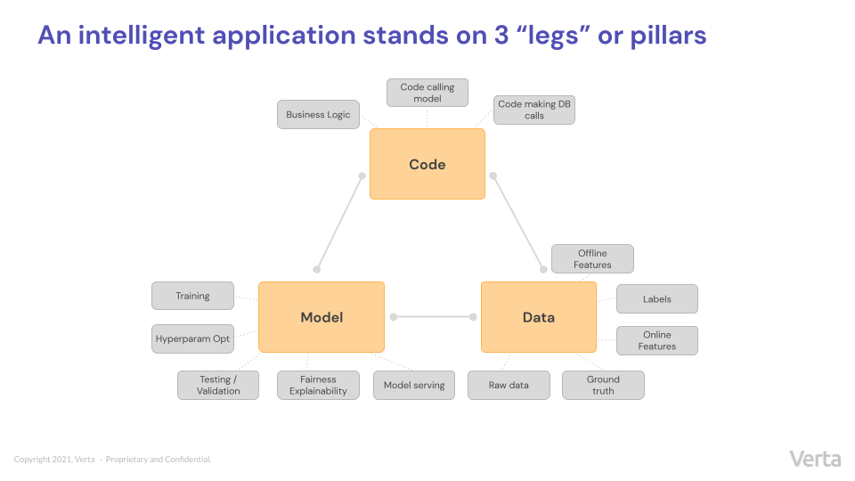
    Intelligent applications are (by their very nature) complex. While conventional software basically consists of one thing (code), intelligent software involves code, models and data. As previously discussed, three distinct fields—DevOps, MLOps and DataOps—have evolved to govern each of these interconnected disciplines. 

    Moving through the ML life cycle quickly and efficiently requires collaboration between teams in each of the above disciplines. Organizations should strive to make this collaboration as frictionless as possible to position their ML efforts for success. What follows are four places where we believe organizations should focus: 

    • Infrastructure
    • Team structure
    • Tools 
    • Project ownership and KPIs

    Build Dedicated Infrastructure for Each Pillar

    Infrastructure software is not one-size-fits-all across the three pillars of code, model and data. For example, DevOps teams have historically played the infrastructure role in software development, supporting application or product services. Think of regular software engineering teams who are supported by DevOps, producing different kinds of application services. App infrastructure is so baked-in to software development that most of us take it for granted.

    Just as regular software services require DevOps, data and model services require corresponding infrastructure. Data infrastructure is typically concerned with managing tools (such as Airflow installations, Spark clusters and feature stores), building data pipelines and ensuring that data services remain smooth and operational for data consumers. 

    On the other hand, model services are chiefly concerned with creating, running and organizing models in such a way that others can use them efficiently. Since the AI/ML life cycle is incredibly complex, a host of factors need to be considered (e.g., hardware, parallelization libraries, model packaging formats, etc.) to help data scientists and engineers do their jobs efficiently. Robust ML infrastructure along with a dedicated ML infrastructure team goes a long way in helping organizations scale their AI.

    Optimize Team Structure

    Best practices for ML and AI are continuously evolving, and organizations have tried a host of team structures over the years. We have noticed two popular structures for intelligent application development teams emerged in recent years:

    • Pods

    Pod structures involve smaller teams—usually a data scientist, a data engineer and an application software engineer—working together closely to deliver an intelligent feature or product. Due to their tight-knit nature, these teams are positioned to iterate extremely quickly, which often leads to better products and features. However, the closely-knit nature of pods also comes with a downside, as knowledge sharing between pods with different objectives can be difficult.


    • Center of Excellence

    In a center of excellence (or COE) structure, all data scientists or data engineers are “pooled” and then assigned to different products or features depending on project requirements and circumstances. In contrast to pods, COE structures tend to share knowledge very easily. However, this arrangement can lead to slower iteration cycles because team members are not dedicated to particular products or features. 

    In our opinion, both pod and COE arrangements can be effective depending on the realities of an organization. Choosing an optimal team structure depends on how the rest of the organization is structured and how reporting relationships are set up. 

    Select Appropriate Tools

    To select the best possible tools for your organization, choose those that foster collaboration and uphold safety across code, model and data teams. 

    The right tools help teams work quickly and efficiently. Teams should be able to discover pertinent information for themselves without having to pull others off of whatever they are working on. For example, a data science team should be able to discover what data access or learn what features exist. Similarly, application teams should be able to discover what models exist, what versions are the latest or how and when to use models. The more that you can make your code, model and data self-serve, the faster teams will be able to build products that are ready to be put into production. 

    Furthermore, proper tools make debugging faster and easier. If you’ve been around ML-enabled features or products for any length of time, you’ve probably been bitten by undeclared dependencies and apps breaking due to upstream changes. In an intelligent app, finding the root of a problem can be extremely difficult because the root cause can exist in any of the three pillars or any combination of the three. Robust tools provide logs and information to help discover what went wrong more easily.

    Finally, governance should play a key role in tool selection, as safety should be a chief concern for ML teams. For example, consider a model that predicts the demographics of a user based on their app usage. While these predictions might be considered acceptable in certain applications, if a model is being used to make financial recommendations or approve credit applications, use of certain demographics may violate various consumer protection laws. Since a software engineer using this model might not be aware of the nuances related to its use, baking in safety checks on model and data use becomes vitally important. 

    Establish Ownership and Determine Appropriate KPIs

    Whether we are working at a company or in an academic lab, our goal always remains the same: build the best product. 

    But “best product” can mean a lot of different things depending on the use case. For example, sometimes teams may be willing to trade a bit of accuracy if a model fails in predictable ways (e.g., in health care applications.) By contrast, an e-commerce recommendation system can optimize for overall model accuracy even if a model isn’t quite as stable. As a result, choosing the appropriate KPIs for model optimization requires careful attention.  

    Similarly, choosing appropriate metrics that make sense for the product and business usually requires a high-level view of a number of factors — user expectations, revenues, user complaints, etc. In our experience, product owners are usually in the best position to make these decisions. KPIs for each of the pillars supporting the intelligent app should be based on key metrics determined by product owners. While these can range, we’ve seen the following KPIs work well:

    • Code — Number of releases, number of bug fixes, number of features that have shipped, mean time to resolution
    • Model — number of model iterations shipped, model quality in production, model performance SLAs 
    • Data — frequency of data refreshes (e.g., every day or every month?), number of data quality issues, speed of access to data

    The key point here is to drive all of these based on the product KPIs and to focus on the agile principle, which is how quickly are you moving and how many deploys are happening. 

    Know what metrics your team is looking to optimize so that you can invest your resources in the right spot. 

  • What is MLOps? DataOps? And Why do They Matter?

    What is MLOps? DataOps? And Why do They Matter?

    Let’s look at three distinct disciplines—DevOps, MLOps and DataOps. In 2011, Marc Andreessen famously proclaimed that software was “eating the world.” A little more than a decade later, it’s all but impossible to argue with his premonition as software has embedded itself into virtually every industry. 

    But now another shift is underway and AI is gobbling up software as we know it. Our emails can finish our sentences for us, connected cars are helping us stay safer on the road and predictive technology is helping minimize supply chain disruptions caused by COVID-19. In the near future, almost every piece of software we interact with will have intelligence built-in, and as AI gains acceptance and new use cases are rolled out, applications will only continue to become more intelligent. The widespread move toward ML-enabled software has the potential to be as transformative and far-reaching as what Andreessen predicted. 

    But innovation is rarely easy or simple—and intelligent applications are no exception. While conventional software involves one thing—code—and not much else, intelligent software relies on a complex relationship between three interconnected variables or legs of a three-legged stool.

    A Three-Legged Stool: DevOps, MLOps and DataOps

    Model:  The one or more AI/ML models (e.g., linear regressions, rules, deep neural networks, etc.) trained to recognize patterns in data and make decisions are what makes an application “intelligent.” 

    Data: Most often, a model is trained on historical data and programmed to emulate it. As a result, an application’s behavior depends heavily on the data—the raw input data, labels and features, as well as the new data to which the model is applied and ground-truth for this data.

    Code: Code is the language an application uses to function. When used in the context of intelligent applications, the code pillar might refer to business logic, calls to models, receiving outputs, decision making and calls to other data systems. 

    A Real-World Example

    To see how these pillars play out in real life, consider the example of a perception system for a self-driving car. Such systems use data (provided by offline sources and real-time cameras and sensors), models and code to determine myriad ever-changing variables (for example, if there are obstacles on the road, what lane markings look like, how fast a car can safely travel, etc.) While the following illustration is greatly simplified, it outlines the basic steps needed to build and deploy such a system and indicates which pillar each step belongs to. 

    Regardless of application type, the legs that intelligent applications stand on are always the same: Model, data and code. And if you try to remove any one of them, the application will topple over.

    With the three distinct pillars that make up intelligent applications, three distinct disciplines have emerged to keep each individual pillar functioning as efficiently as possible: DataOps, MLOps and DevOps. The rest of this post examines the details that make each discipline distinct and necessary to the model life cycle.

    DevOps

    Once upon a time, companies used waterfall processes to develop software. The process often moved so slowly that products didn’t realize their potential before they died or were replaced. In 2000, Agile was introduced, allowing developers to work quickly and iteratively in tight sprints where they were constantly delivering. By 2009, Flickr, for example, was the envy of the industry, routinely performing 10+ deploys per day. Companies seeking to increase their own productivity combined software development with established operations principles—and the term “DevOps” was coined. 

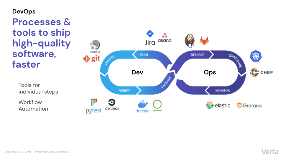
    As the familiar loop graphic below illustrates, the DevOps cycle goes from the planning stages to the creation, testing/verification, packaging, release, configuration, monitoring and then starts over again with planning. Over the past two decades, a host of unique tools have emerged to support individual steps in the DevOps life cycle—helping developers ensure quality by building in continuous integration and continuous testing from the start and helping speed up time-to-market with workflow automation. The DevOps ecosystem is robust, well-thought-out and always iteratively improving.

    MLOps

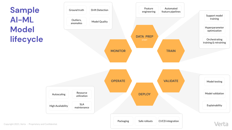
    MLOps helps teams move more quickly and efficiently through the model life cycle—a loop that involves six distinct steps, each of which contains unique considerations. 

    Since MLOps is related to DevOps, businesses sometimes try to adapt the processes used to write conventional software to execute the unfamiliar task of machine learning operationalization. But the approach doesn’t work, as the two disciplines are actually quite different.

    MLOps primarily deals with models, not code—and models are quite different from code. For example, model training and testing look very different from code building and testing. (What does “test case” even mean for a model?) And monitoring model performance is completely different than monitoring traditional software. (DevOps looks at things like CPU utilization, latency and throughput, while MLOps looks at model quality, drift and data quality.)

    Furthermore, the people that MLOps engineers are building for are quite different than their DevOps counterparts. As one might expect, the primary users of models are data scientists while DevOps generally serves software developers. Most often, MLOps engineers come from a background in ML and data science or software engineers who picked up ML. 

    As with DevOps, no single all-inclusive MLOps platform exists. Rather, different tools support different individual steps in the model life cycle and provide some amount of workflow automation to speed up processes. Different tools support specific pieces of the ML life cycle—but the ecosystem is still somewhat fragmented. Ideally, MLOps will evolve to offer more DevOps-like tools that work well together and offer more automation. For companies looking to build an MLOps platform, build a suite of supporting tools with speed, safety and automation in mind.

    DataOps

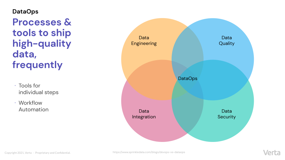
    We’ve seen very well-defined life cycles for the other two pillars discussed above; however, when it comes to DataOps, the life cycle is still being defined. But the overall objective of DataOps should sound familiar: DataOps involves processes and tools to ship high-quality data frequently—which requires a combination of data engineering, data quality, data security and data integration. 

    As with DevOps and MLOps, what the DataOps platform or DataOps engineer is doing is supporting the tools that help perform one of these activities and help build workflows. For example, a workflow may take data from a database, apply some transformation to it and then make it available for a business intelligence (BI) tool. That’s the kind of automation that is involved in DataOps. 

    As you might imagine, the skillset and the tools required for DataOps are quite different from the ones needed in MLOps and DevOps—so expecting a DevOps engineer to also be an expert in DataOps seems a bit unrealistic. While MLOps requires a much tighter integration with data than DevOps historically has required, MLOps is not the same thing as DataOps. More so than the other pillars that support intelligent applications, DataOps tends to be quite separate and distinct. 

    Conclusion

    From perception systems to enterprise-scale fintech software, every intelligent application depends on three distinct disciplines: DevOps, MLOps and DataOps. And therein lies the complexity of developing intelligent products. Each of these fields is distinct, dealing with a different set of questions and objectives within the ML life cycle and requiring different kinds of people and tools. However, they are all fundamentally united by a common goal: Optimizing quality and speed of iteration of the ML life cycle. The tools, practices and organizations that will rise to the top are the ones that will enable more seamless collaboration between different ML teams, helping them move through the ML life cycle quickly and efficiently. 

  • SQL Server MDF to NDF Distribution

    SQL Server MDF to NDF Distribution

    Do you have massive MDF files on your database? Have you noticed that your SQL Server disk stall metrics for these data files are higher than the storage latency metrics exhibited on the underlying operating system? It could be that your SQL Server data files are being hammered too hard and you don’t have enough data files to help the SQL Server storage engine distribute the load. We do this for tempdb, right? Let’s do this for our user databases as well. It’s easy for a brand-new database. But existing databases may be out of control with a single data file. Let me show you how to adjust this for existing databases without an outage!

    I’ll be taking the SQL Server database generated by the HammerDB benchmark, appropriately named tpcc_test. It’s just a backed-up-and-restored copy of the (appropriately named) database tpcc_single to represent a single MDF file present. 

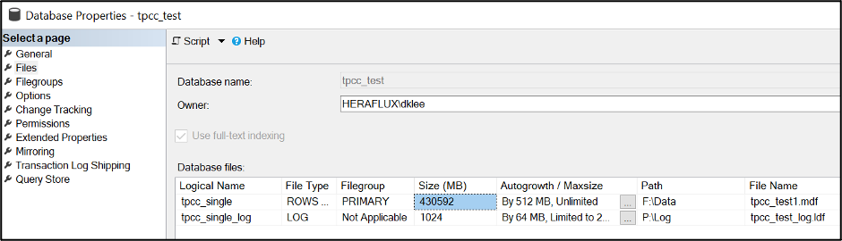
    I did a restore onto the F: drive of this server. The MDF size is rather substantial at 420GB. The log size is inconsequential for the purposes of this task.


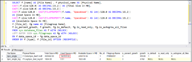
    Here’s the interesting part. Take a look at the current file system size versus the internal fill size. Record the internal fill size, as that’s what we’ll be using to help with some math shortly.

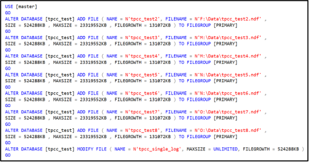
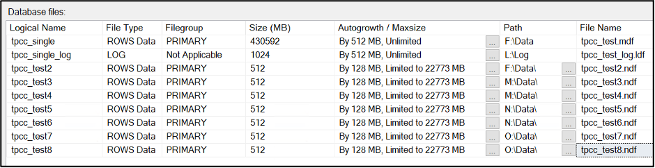
    Now, how many files do you need? Here’s my standard DBA response—it depends. For the purposes of this test, I’m going to add seven NDF data files to complement the primary MDF. Your mileage may vary based on your workload. 

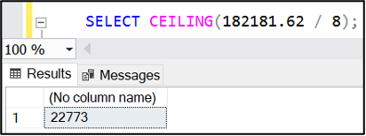
    How large do these files need to be? Take the internal fill size on the MDF, divide by the number of data files you want in total and round up to the nearest megabyte. If the database is active with a lot of data being added, you might want to add a bit more just to have it balance by the time we’re done with this task.

    SELECT f.name AS [File Name] , f.physical_name AS [Physical Name], 

    CAST((f.size/128.0) AS DECIMAL(15,2)) AS [Total Size in MB],

    CAST(f.size/128.0 – CAST(FILEPROPERTY(f.name, ‘SpaceUsed’) AS int)/128.0 AS DECIMAL(15,2)) 

    AS [Available Space In MB], f.[file_id], fg.name AS [Filegroup Name],

    f.is_percent_growth, f.growth, fg.is_default, fg.is_read_only, 

    fg.is_autogrow_all_files

    FROM sys.database_files AS f WITH (NOLOCK) 

    LEFT OUTER JOIN sys.filegroups AS fg WITH (NOLOCK)

    ON f.data_space_id = fg.data_space_id

    ORDER BY f.[file_id] OPTION (RECOMPILE);

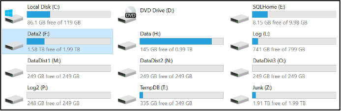
    Now is the time to determine if these should be placed on the same disk or if they should be distributed across more disks. I’m doing that on this server to leverage the disk controller queues to more widely distribute the storage activity and see better overall performance when under pressure. I’ve attached three more virtual disks to this virtual machine, and the four are spread on the four disk controllers on this virtual machine. All disks are formatted with a 64KB NTFS allocation unit size with the large FRS flag enabled. Let’s place two of these files on each disk with the fourth holding the last NDF with the MDF. 


    Here’s a trick: I set the maximum file size of each of the new NDF files to be the percentage of the current main file space consumed. 

    Now, we’re going to use a little-known command to empty the MDF file. It’ll drain the file completely, but since we capped the file growth of the NDF files that we attached to limit their growth rate, this command will run until we have filled the NDFs, then fail. It will take longer to perform this operation, but it keeps the database online while it runs. You might have a bit of a performance hit from the CPU and I/O impact of this running process, so it’s important to think about timing when running this operation.

    You can watch the process work with the internal used space query listed above; the primary MDF is draining while the other NDF files are slowly filling up.

    Again, it takes time for this process to finish. When it finally ‘completes’, the EMPTYFILE command will fail due to maximum file size limit on the NDF files.

    FYI—Index optimization routines can cause a circular block with this process that I have encountered twice while running this process, so keep an eye out if you see this occur.

    Now, your internal data consumed space rates are almost identical. 

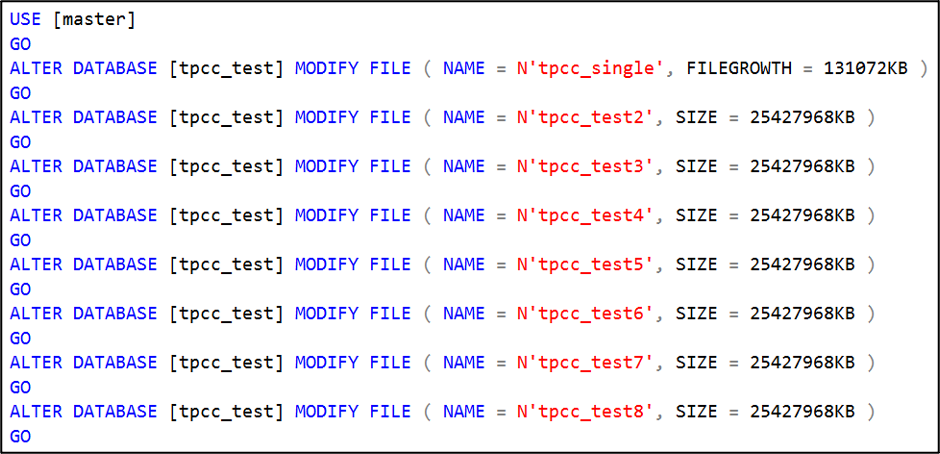
    Verify the autogrow rates are now the same between the data files. Remove the file growth limit on the NDF files. 

    Perform a one-time shrink of the primary MDF file to shrink it down to where it is the same size as the others.

    It will most likely be slightly out of balance. SQL Server does a pretty good job with the round robin algorithm for internal file fill rates, and it will finish balancing and then round robin filling internally as you continue to add data through normal usage. If you need to increase the size on some of the files so they match, go for it, and SQL Server will fill accordingly so it finally balances.

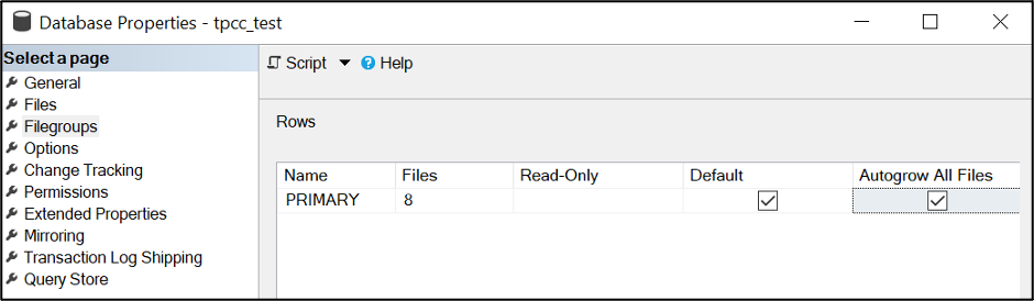
    You might also check if you need to enable autogrow all files at the same rate. This could mean that the database users might need to be punted from the database to enable the change.  Do this during a maintenance window.

    Sample your SQL Server disk stall rates and see what different you experience once this goes live.

    I hope this helps you improve the operational efficiency of your SQL Server database data files, and you get better performance as a result. Let me know how this works for you!

    Update: If you encounter an error like the following, just shrink the main MDF file down and repeat the emptyfile operation.

  • DevSecOps for Databases: Data Masking, Cloud Backup, WAF and More

    DevSecOps for Databases: Data Masking, Cloud Backup, WAF and More

    DevSecOps is everywhere. More and more organizations realize that the traditional separation between DevOps and security is wasteful and dangerous. As a result, they are rushing to integrate security into all their software development processes. 

    Adding security to containerized applications, cloud resources and other parts of modern DevOps infrastructure is already well understood. But what about databases? Databases were always—and remain—a critical system component and a prime target for attackers. Here, I’ll review the basics of modern database security and show you how to create a continuous security process for databases in a DevSecOps organization.

    What is DevSecOps?

    DevSecOps incorporates security practices into the DevOps methodology. DevSecOps promotes a ‘security-as-code’ approach via the partnership between release engineers and security teams. Similar to DevOps, the DevSecOps approach focuses on creating innovative solutions for complex software development processes. Teams complete this within the framework of an agile approach.  

    DevSecOps aims to close the gap between security and IT teams while ensuring the speedy and safe delivery of code. Organizations replace the siloed development method with a new approach that promotes the shared responsibility of security tasks during the delivery process. 

    In DevSecOps, two supposedly opposite aims—delivery speed and secure code—are united into one effective process. 

    Database Security Basics

    The term “database security” is an umbrella term used to describe all of the tools created to develop and preserve database availability, integrity and confidentiality. A key responsibility for any DBA is to ensure that the information stored in databases is always secure.

    The goal of database security is to protect:

    • Database management systems
    • Applications that access database information
    • Datastores within databases
    • Hardware servers
    • Virtual database servers, such as cloud-based servers
    • Network access points

    It is critical to strike a balance between security and usability. While you must prioritize data security, information needs to be accessible to offer value to the organization. The more access you provide to the information retained in a database, the more vulnerable the information is. However, an overly secure database is neither practical nor functional.   

    A good way to achieve a balance between accessibility and security is to create meaningful security protocols, create tiered levels of information access and invest in a robust database security and activity monitoring tooling. 

    Common Threats and Challenges

    Here are some of the most common types of database attacks:

    • Insider threats—These involve privileged users misusing their access credentials. An insider could be a negligent employee who unwittingly exposes the database to attack, a malicious insider who abuses the database on purpose or an outside infiltrator who steals credentials to breach the database. The risk of a breach increases as more employees hold privileged access credentials.
    • Injection attacks—These involve inserting arbitrary attack strings into the database queries that HTTP headers or web applications serve. These attacks can be SQL or NoSQL. Secure coding practices and regular vulnerability tests should help protect you against injection attacks.
    • Database software vulnerability exploits—Database software providers regularly release security patches for vulnerabilities in their software. However, if you don’t apply the patches quickly, you prolong your exposure and run the risk that hackers will exploit vulnerabilities in your database. 
    • Backup attacks—If you don’t protect your backup data with sufficient controls, you expose your database to an attack on your backups. 

    The following challenges can exacerbate these threats:

    • Large volumes of data—Organizations must adequately manage increasingly large volumes of data using scalable tools and practices.
    • Sprawling infrastructure sprawl—Organizations are increasingly shifting to hybrid and multi-cloud environments, making their networks more complex and security harder to manage. 
    • Evolving regulations—With the global regulatory landscape changing and growing more complex, it is increasingly challenging to maintain compliance.
    • Skill shortage—The demand for cybersecurity personnel far outstrips supply, and this shortage is only likely to increase in the future. 

    4 Techniques for Continuous Database Security With DevSecOps

    A DevSecOps approach calls for continuous database security during all stages of database development and usage. Let’s explore a few techniques for achieving continuous security.

    Data Masking

    Data masking technology lets you create a structurally similar, anonymized version of an organization’s data. You can use this data for user training or software testing. The aim is to safeguard the real data while using a functional substitute for use cases in which the actual data is not needed.  

    In data masking, you keep the format of the data the same. You only change the values of the data. You can alter the data in various ways including character shuffling, encryption and word or character substitution. Whichever method you choose, you have to modify the value in some way that makes reverse engineering or detection impossible. 

    Use data masking when presenting data to users (whether inside or outside the organization) who don’t need to access the data as part of their role. You should apply data masking to all sensitive information before displaying it in public forums. 

    Use Web Application and Database Firewalls

    Protect your database server from security threats using a firewall that stops access to traffic as a default. The only traffic permitted should come from particular web servers or applications that require access to the information. The firewall must also prevent your database from establishing outbound connections unless they are specifically needed. 

    Protecting the database using a firewall is not enough. You should also deploy a web application firewall (WAF). That’s because SQL injection attacks, which target web applications, can be employed to delete or exfiltrate data from the database. A database firewall may not stop this from occurring if attacks are initiated from an application that is a permitted source of traffic. However, a web application firewall likely will stop attacks of this nature because it can analyze traffic at the application layer and identify malicious query patterns.

    Cloud Backup

    Database backup solutions help organizations safeguard their data with backup database copies in the event of user error, physical hardware failure, data corruption or ransomware attacks. Organizations can ensure their information is always accessible by using database backup tools, even if their central database fails or is compromised. 

    Cloud backup services allow you to send a database copy to an off-site, secondary location for safekeeping if there is a disaster or failure. A third-party service provider typically hosts the secondary data storage systems and servers. This provider bills the backup customer based on capacity used or storage space, number of users, data transmission bandwidth, number of times the information is accessed or the number of servers. 

    Using cloud data backup can help you improve data protection without overwhelming IT staff. This labor-saving advantage could be significant and may even offset some of the added costs connected with cloud backup, including data transmission costs. 

    Secure Database User Access

    You must strive to limit the number of individuals with access to the database to the extreme minimum. Administrators should only have minimal privileges—those they require to carry out their job and only when they require access. 

    For small organizations, this might be difficult to achieve because employees have multiple roles, and there may be only one or two database administrators. However, you should at least manage permissions using roles or groups rather than granting access directly.  

    If you have a large organization, you must think about automating access management via access management software. Access management software can give authorized users a provisional password with the privileges they require every time they want access to the database. This software also logs the activities conducted during that time and stops administrators from sharing their passwords. 

    It is critical to lock down any form of password sharing—this is a common practice by administrators and database users, but it makes accountability and effective database security nearly impossible. 

    In addition, you should follow standard account security procedures: 

    • Enforce the use of strong passwords
    • Store, encrypt and salt password hashes
    • Lock accounts after three or four login retries
    • Deactivate accounts when employees leave or switch to different roles

    DevSecOps and Database Security

    In this article, I explained the basics of DevSecOps and database security, covered the primary threats facing database systems in a modern IT environment and provided four ways you can implement continuous security for databases:

    • Data masking—All modern RDBMS systems offer data masking mechanisms that can reduce the impact of compromised accounts.
    • Using WAFs and database firewalls—Firewalls provide excellent runtime protection and visibility for application-layer attacks.
    • Cloud backup—Backing up databases in the cloud is a continuous process that can enhance availability and reduce the impact of ransomware attacks.
    • Secure database user access—Using least-privilege principles can dramatically reduce the threat surface of a database.

    I hope this will be useful as you extend your DevSecOps practices to critical database systems in your environment.

  • Why DataOps is Critical for Digital Transformation

    Why DataOps is Critical for Digital Transformation

    Data lies at the heart of all digital transformation. In fact, today, as organizations look to further accelerate their ongoing digital transformation initiatives, companies are looking to extract even more value from their data, to better drive corporate decision-making, help grow the business, improve customer satisfaction and gain a competitive advantage. 

    Inspired by DevOps, DataOps, which Gartner defines as “a collaborative data management practice focused on improving the communication, integration and automation of data flows between data managers and data consumers across an organization”, has grown in popularity in the past decade as organizations seek to accelerate the delivery of business value from their data. But taken even one step further, enhanced data operations (i.e. more than DataOps) can help organizations maximize the business value of the data they own and also the infrastructure in which the data resides to increase data quality, reliability and availability in a hybrid cloud environment. This enables organizations to further improve business resilience and digitalization through collaborative, data-centric operations in an increasingly complex, interconnected world. Particularly as hybrid and multi-cloud environments proliferate and it becomes harder for teams to understand, analyze and streamline data usage.  

    DataOps Enables Digitalization

    By 2023, IDC predicts that 52% of worldwide GDP will come from products and services delivered by digitally-transformed enterprises—and according to Gartner, 91% of enterprises are already involved in some sort of digital initiative. This means that organizations already engaged in digitization are paving the way for a new future of business—commerce, production and innovation. But digitization is only half the battle—the other half (i.e., digitalization) comes from investing in understanding those digitally-driven insights and using those learnings to fuel business growth. 

    In the face of stifling market competition and evolving customer demands, the key differentiator in market leadership today is data and operationalizing that data. Hence, the difference between the market leaders and followers boils down to this: Data operations. Data operations not only plays a vital role in empowering ongoing digital transformation initiatives (think hybrid cloud operations, DevOps optimization and application modernization; data is at the core of all of these efforts) but also serves as a foundation for faster, better-informed innovation—fueling organizational growth and propelling businesses ahead of their competition.

    Who is Driving Digitalization?

    To gauge where your organization stands on your digitalization or digital transformation roadmap, you must first identify who within your organization is driving it and who’s involved. The latter is an easy enough guess—because, essentially, it’s everyone. 

    Although digital transformation is defined as the transformation of the digital operations of an organization, it reaches far beyond IT to all major functional departments and requires a cultural change to reach its fullest potential. That includes everyone from the chief information officer (CIO) and chief data officer (CDO)—collaborating with key stakeholders to map out and define digital transformation strategies and efforts and communicating goals and objectives—to the technical and professional teams—working closely with business units to design and operationalize new architectures and technologies to advance digital transformation initiatives. At the core of all of these modernization efforts is data; the metric for business success in the digital age. As such, integrating DataOps into your digital transformation efforts from the start is mission-critical. 

    As the market becomes increasingly competitive and business leaders look for new ways to grow and expand their business, data will remain a key catalyst in achieving those lofty digital transformation goals. By gaining intelligence from their data, companies can realize the ultimate goal of data empowerment—where all employees have simplified, secure levels of access to the high-quality data they need to do their jobs—enhancing operational efficiency, improving business outcomes and fueling business transformation at scale. 

  • How to Pivot and Join Time-Series Data in Flux

    How to Pivot and Join Time-Series Data in Flux

    Merging multiple time-series in InfluxDB using Flux may seem like a daunting task. This in-depth Flux tutorial will explain how to pivot, time shift and join time series in InfluxDB.

    In this InfluxDB tutorial, we will show you how to create an accurate overview of multiple time series with industrial data captured in consecutive production steps. Doing this requires a proper join mechanism for combining the time series into one after aligning them with respect to time.

    This tutorial is based on a real-world case we solved at Factry.io with InfluxDB in an industrial setting.

    Every second of the day, production sites all around the world are generating inconceivable amounts of process data. This data is directly acquired from production lines on-site and captured in the form of process parameters. Being able to reliably keep track of these process parameters throughout the production process is essential to continuously improving manufacturing operations.

    Industrial process parameters are represented as concurrent time series. They do not necessarily provide data points at a similar pace, nor are they always aligned over time. Obtaining a trustworthy overview of captured process parameters during consecutive production steps can be daunting.

    Time-Series Data Explained

    In brief, time-series data represents a number of different data points indexed by time. As time is a constituent of anything that is observable in our world, time-series data is everywhere. When narrowed down to a production environment, captured process parameters are distributed in time in order to become distinguishable from the process data preceding or following it.

    What is the difference between time-series and relational data? In contrast to time-series data, relational data holds records that are generally referenced by an artificial identifier. These identifiers can interrelate, which crafts the relational aspect.

    Pivot and Join Time-Series Data in Flux

    Before you get started

    On a production line, be aware that a product batch cannot be in two different production steps at the same point in time. As a result, time series measured in different production steps are naturally unaligned. Hence, before properly joining these time series into one, many of them will need to be shifted over time to get the overview right.

    Furthermore, retrieving data stored in a time-series database is commonly done by using the dedicated query language Flux.

    Two points about this:

    1. In Flux, a join can only make use of an inner join mechanism to melt multiple time series into one. As an inner join solely retains the data points for shared timestamps in multiple time series, data loss is unavoidable when dealing with unaligned time series or time series captured at different rates.
    2. In most use cases, only time series extracted from sensors at different production steps need to be joined. This is due to the ability to differentiate between multiple tables within one time series.

    Hence, reading in sensor data generated by multiple sensors at the same production step, table by table, allows us to bundle the sensor data. By ‘pivoting’ the tables into one, a time series is forged. Prior to being joined with the sensor data captured from another production step, the time series is shifted to align with respect to time. However, note that this requires all sensor data (potentially from different sensors) from one production step to be aggregated in the same way, omitting any differences in the rate at which it has been captured.

    Use Case: Welcome to the Cardboard Factory

    There are some best practices for pivoting and joining time series data in Flux from consecutive production steps. In this example, sensor data is captured from a replicated production site that is manufacturing cardboard panels out of recycled paperboard rolls.

    The production process of the cardboard factory consists of three different steps, which we’ll refer to as entries A, B and C.

    • In entry A, production starts with recycled paperboard rolls; the width and diameter of which is being measured by two separate sensors.
    • In entry B, the recycled paperboard rollsare cut into paperboard sheets and processed into cardboard using a certain temperature and pressure.
    • In entry C, the cardboard is cut into shape. For this entry, the height and the thickness of the panels are the key elements to be measured in terms of sensor data.

    With respect to time, it takes approximately one minute for the first sheet of recycled paperboard roll to reach entry B. Further, about two minutes elapse before the paperboard sheet is processed and shaped into a cardboard panel.

    Note that, in this production site, it is assumed that the speed of the production line is more or less fixed over time, making it possible to shift time series captured in different entries in order to get them aligned.

    Merging Multiple Time Series Into One Using Flux

    The goal in this use case is to create one trustworthy overview of all sensor data captured in each entry. Imagine today is May 4 at around 3:10 p.m. The overview should be reflecting all sensor data from the past ten minutes of the production site.

    Fortunately, we are aware that the sensor data between each entry is unaligned by a few minutes. Therefore, we should be fetching data between 3:00 and 3:10 with respect to the last entry (entry C); thereby trying to align these time series with the ones from both entry A and entry B.

    Think about it as being teleported to 3:10 on May 4. At that time, for a recycled paperboard roll in entry A or for a paperboard sheet in entry B, we do not yet have the sensor data for entry C. This is obviously because this sensor data will be captured only a few minutes later on the line.

    With this cleared up, a recycled paperboard roll delivered by one of the suppliers is referred to in the use case as a material lot. In contrast, a paperboard sheet derived from the recycled paperboard roll resulting in a cardboard panel is mentioned as a material sublot.

    At the end of the production line, a pile of cardboard panels is manufactured out of one material lot. To sum it up: In this use case, a material sublot can never be in two different entries at the same point in time, which means we need to align time series over consecutive entries.

    1. Reading in the Sensor Data

    First, we start by reading in the sensor data of both the width sensor and the diameter sensor for entry A. By reading in sensor data of both sensors in the same ‘filter’ (image: code snippet), we reduce this data to one time series for entry A.

    In this way, we hold different tables per sensor in one time series arranged by the group key consisting of ‘_field’ and ‘_measurement’. By reducing all sensor data from one entry to one time series holding multiple tables, the opportunity arises to pivot the tables into one unified table later on.

    Fetching the corresponding sensor data from entry A with respect to entry C is fulfilled by using a ‘range’ with sensor data that was captured between 2:57 and 3:07. This is applied by shifting the time range of entry A three minutes backward using ‘SHIFT_A’. Hence, for a cardboard panel at entry C, the corresponding sensor data at entry A was captured three minutes earlier.

    In essence, we are mapping the time range between 2:57 and 3:07 of entry A onto the time range between 3:00 and 3:10 of entry C and, thus, onto the overview.

    Note that for operations between a timestamp and a duration in ‘FROM_A’, you need to convert both the timestamp and the duration to an unsigned int to get Unix timestamps in ns prior to performing the calculation.

    Entry A sensor data – code snippet

    Entry A sensor data

    Regular and Irregular Time Series

    In most use cases, the sensor data will generate a regular time series (metrics), as the time period between captured data points will be fixed. However, when working with irregular time series (events) or time series generated at a different rate, these need to be transformed into a regular time series with an ‘aggregateWindow’ to eventually build up a nice overview.

    In this use case, there is only a regular time series. Therefore, retaining the ‘last’ data point for each time window of one minute should do the trick. In the case of an irregular time series, taking a ‘mean’ over a fixed time window would be the better choice.

    2. Pivoting the Time-Series Data

    After the sensor data from both sensors of entry A is collected into one time series with multiple tables, we now need to pivot the tables to become one. Therefore, the group key of each table needs to hold the same schema.

    In this use case, the group keys schema for all tables in the time series is as follows: ‘[‘_field’, ‘_measurement’]’. To make sure that the group keys schema is identical for all tables, we can use a ‘keep’ in front of the pivot to eliminate fields that are not present in all tables.

    Possible Deal-Breakers

    Bear in mind that the constraint for holding an identical schema for each table in the time series can be a deal-breaker for using the pivot. Another constraint lies in the lack of being able to pivot more than one value field, although when reading in sensor data from InfluxDB, there is typically only one value field.

    However, after adding some processing to the time series in Flux, chances are that an additional processed value column is present, eliminating the ability to use a pivot once more.

    When performing a pivot on multiple tables in the time series of entry A, for the table rows holding a shared timestamp (row key: ‘_time’), the data point in the value field (value column: ‘_value’) will be ingested into a column determined by the name of the measurement (column key: ‘_measurement’).

    In the use case, this means that the tables with the measurements ‘lot_ID’, ‘A_width’ and ‘A_diam’ will get their data points from the ‘_value’ field ingested into a separate column in the unified table, determined by their measurement names.

    In terms of performance, a pivot can suffer from having too many tables in the time series to be pivoted, which corresponds to the number of active sensors in one entry. Next to that, an extensive group key schema in the pivot will also take its toll. Having a considerable amount of rows per table in the time series of an entry with ns precision timestamps can easily blow up the pivot, as well.

    Finally, a small footnote on the functionality of the pivot in Flux. Keep in mind that the fields and tags that are not included in the pivot will not be ingested into the unified table. Additionally, the term pivot appears deceiving when being compared to its functionality in a relational database.

    Entry A pivot – code snippet

    Entry A shift


    3. Time Shifting the Time Series Data

    Entry A

    After pivoting the sensor data of entry A into one unified table, the entry A sensor data with time range between 2:57 and 3:07 gets aligned with the time range of the overview between 15:00 and 15:10 by performing a time shift of three minutes forward on the _time column.

    To preserve the original timestamps of entry A, we take a duplicate of the _time column in the unified table and refer to it as the time for which a sublot actually started at entry A, mentioned as entry_A.

    entry A shifted – code snippet

    Entry A Shift – Code Snippet

    Entry A Shift

    Entry B & C

    The same procedure for reading in the sensor data of entry A applies for entry B and entry C. While the sensor data for the former is shifted by two minutes to get its time range between 2:58 and 3:08 aligned with the time range of the overview, the sensor data of the latter is already in sync for the overview.

    Entry B – code snippet


    Entry B

    Entry C – code snippet


    Entry C


    4a. Joining the Time Series

    After pivoting the sensor data for each entry, three distinct time series are held, each containing one table with a separate schema and multiple value columns; for example, ‘C_height’ and ‘C_thickness’ for entry C. To create one overview, these three time series must be joined together, visualizing the data points of different sensors side-by-side with respect to time. Since the sensor data of the different entries has been formerly aligned by reading in the corresponding time ranges for each entry followed by a ‘timeshift’, the three time series can now be joined on the synced ‘_time’ column present in each of them.

    Possible Issues

    Since the schema differs between the three time series tables, you would encounter significant overhead when trying to pivot these three tables into one after appending them to a single new time series. Besides the superfluous complexity added, the tables of all time series are each holding more than one value column, which makes the pivot unusable in this case.

    A plausible solution would be to use a ‘join’ provided by Flux on the aligned ‘_time’ column. As discussed in the pivot and join section, the ‘join’ is represented as an inner join mechanism, solely retaining data points for shared timestamps between joined tables.

    In this use case, the inner join mechanism would not trigger any data loss, since only regular and aligned time series are present after the pivot. However in case of irregular time series (not using ‘aggregateWindow’ on events), time series captured at a different rate or regular yet unaligned time series, data points would get lost in the inner join mechanism.

    Next to that, the ‘join’ in Flux is only letting two time series be joined together at once, which constrains the possibilities. Moreover, seen from a performance perspective, the ‘join’ is considerably less optimized compared to dedicated functions in Flux, like the ‘aggregateWindow’.

    4b. Solution: Outer Join

    To tackle the issues subject to the ‘join’ provided by Flux, an outer join mechanism is proposed, retaining data points for both shared and unshared timestamps between tables of multiple joined time series with respect to time. After appending the three time series to a single new time series holding one table, the outer join mechanism groups all data points by time into ‘timetables’ prior to filling up rows with the appropriate data points. Furthermore, the single complete row per timetable is extracted, preceding the ungrouping of timetables to one overview table.

    Union

    Once the aligned sensor data is available into a dedicated time series per entry consisting of one table, the three time series are appended by a ‘union’ to a single new time series holding one table. The ‘union’ is ingesting the sensor data of each entry vertically (image: union), meaning the table rows per entry are placed underneath each other while the resulting table schema is the union of the separate table schemas of the three time series. In this manner, you can witness ‘data point blocks’ in the resulting table referring to sensor data of each entry in the production site. Note that the ‘union’ allows more than two time series to be appended to a new single time series at once.

    union – code snippet

    union


    Timetables

    The sensor data of all three entries in the single time series table is grouped by the ‘_time’ column to group the sensor data of different entries together in timetables. The ‘timetables’ refer to the tables that arise by using the group key ‘_time’ (image timetables). The forthcoming sort is fundamental to order the rows of a certain entry at the bottom of a timetable prior to starting to fill data points. In this use case the row originating from entry C is positioned at the bottom of each timetable’ by sorting for the ‘entry_C’ column in ascending order. In fact, regardless of sorting the ‘entry_C’ column in ascending or descending order, the empty data points in the ‘entry_C’ column of the rows originating from entry A or entry B will always be on top in Flux since they hold a null value.

    Timetables – code snippet

    Timetables 

    Fill

    Moving forward, the data points of the columns originating from entry A and entry B are copied into subsequent rows using the ‘fill’ with ‘usePrevious’ set to ‘true’. Since the data points are filled through the bottom, the mutual order of the rows originating from entry A and entry B is not important. Note that at the bottom of each timetable, the row originating from entry C is now a complete row holding all data points for all three entries (image: fill).

    fill – code snippet 

    fill

    Extract

    Finally, only the complete row at the bottom of each timetable is extracted by using the ‘tail’ with ‘n’ set to ‘1’. The timetables are ungrouped to one joined table by using the ‘group’ without any parameters to empty the group key. Check out the joined table (image: extract) and you’ll see that all sensor data originating from the three entries of the production site is visualized into one trustworthy overview with respect to the time behavior induced by a sublot passing through the production entries on site.

    Extract – code snippet 

    Extract


    4c. Outer Join Mechanism for Unaligned Sensor Data

    To illustrate the outer join mechanism, one can join unaligned sensor data for the corresponding time ranges from the 3 entries in the production site into one overview. This can be arranged by removing both the ‘timeShift’ of three minutes for entry A and the ‘timeShift’ of two minutes for entry B when compared to entry C.

    In that case, the sensor data of entry A will retain its time range between 2:57 and 3:07, while entry B will have a time range between 2:58 and 3:08, followed by a time range between 3:00 and 3:10 for entry C. The result is a broader overall time range for the overview than requested (image: outer join on unshifted sensor data). Besides, only unaligned sensor data is present for all three entries in the time range between 3:00 and 3:07.

    Note that for the top and the bottom rows, the unavailable sensor data for a certain entry is replaced by the ingestion of null values as data points in the columns are originating from the corresponding entry. As mentioned earlier, the same principles apply for an outer join when dealing with irregular time series or time series captured at a different rate. Ideally, such an outer join mechanism should be the default behavior in Flux when performing a ‘join’.

    Outer join on unshifted sensor data 

    Conclusion

    When creating a trustworthy overview of captured sensor data at a production site in consecutive production steps, take these four elements into account:

    1. The step in the production process where the sensor data is captured is key to understanding the time behavior of a product batch going through the different production steps on site.
    2. How sensor data is captured in production indicates the urgency of using a specific time window and which selection/aggregation of data points you should obtain. Hence, sensor data can generate a regular or irregular time series or can be captured at a different rate.
    3. Sensor data per production step is pivoted to a time series holding one unified table of sensor data for that production step. The pivot stands out in unifying the sensor data per production step, since the different tables each referencing a sensor in that production step typically hold an identical schema when reading them in.
      • Next to that, generally speaking, there will only be one data stream per sensor and thus only one value field per table in the time series derived from a production step.
      • Performing an outer join on the multiple time series originating from multiple production steps, gives you the ability to create a trustworthy overview in the end. To make the most out of it, make sure to align the time series first before joining them.
  • DataOps: How to Turn Data into Actionable Insights

    DataOps: How to Turn Data into Actionable Insights

    Enterprises‌ ‌have‌ ‌struggled‌ ‌to‌ ‌collaborate‌ ‌well ‌around‌ ‌their‌ ‌data, which can impact everything from digital transformation to advanced concepts like AI and ML.‌ ‌DataOps is not without challenges; building, managing and scaling data pipelines requires careful thought around reusability, portability across infrastructure and applications and long-term maintenance and governance. And these are just a few of the issues facing enterprises. For this reason, DataOps technology stacks need to focus on providing key capabilities include data extraction, integration, transformation and analysis.

    The Importance of DataOps

    The enterprise is undergoing a seismic shift from siloed application development and data repositories to more composable and reusable architectures. Additionally, there is a growing demand for speed and agility as well as the influx of disruptive technologies such as the cloud, IoT and AI. Organizations that want to win big must act and adapt quickly to deploy and scale new software and solutions that provide customers with a superior experience and satisfy their rapidly evolving needs. To do that, they also must be able to rapidly aggregate, integrate and analyze data sources.

    Even with this need for speed, the tools and processes for the creation and processing of data are not standardized‌ in‌ a way that promotes rapid innovation‌ and ultimately helps organizations transform. DataOps is critical to address the challenges involved in acquiring, storing and governing data. In addition, companies are dealing with increasing complexity in their IT environments. In a recent survey, more than 80% of enterprises have a hybrid cloud or multi-cloud strategy. In order to have cost-effective and secure management of increasingly large amounts of data, enterprises must adopt DataOps.

    Managing Data Growth

    DataOps has been around for about a decade, but has recently gained momentum because of the overwhelming challenges companies face today in dealing with large, complex sets of data that are being generated at increasingly faster rates. With new technologies like the internet of things (IoT), cloud computing and the power of big data now integrated into everyday use, companies are generating at least 50 times more data than they were just five years ago. And with more data comes a need for greater efficiency and higher demand for data experts.

    DataOps potential impact on businesses might lead you to think of it as a radical new methodology. But many companies have already been using similar practices to deal with some aspects of data management, particularly around data warehousing and analytics. And just like DevOps, DataOps isn’t a product, but rather a cultural shift supported by many products—many existing products. So it’s important for businesses looking to adopt DataOps to consider what they already have, such as enterprise data warehouses and ETL tools, and what they may need to acquire, replace or modernize. In the end, companies will end up with several systems to support the data pipeline.

    DataOps and Big Data Challenges

    Most enterprises have invested in significant data infrastructure to extract, load and store their data to take advantage of Big Data analytics and technologies. However, these infrastructures are often layered, hard to manage and full of legacy tools that hinder the transfer and integration of data. Additionally, organizations have invested significant resources in tools such as data warehousing and data marts. These data warehouses have been used to model data but have been typically implemented with a predefined data model. A business intelligence (BI) system, an enterprise data warehouse or any other set of tools might assist in the execution of a data transformation job.

    The technological revolution is creating unprecedented opportunities to make things happen with data. By analyzing the data that powers modern business, we are able to provide value in every dimension of our organizations. As is the case with every transformation, the benefits of building an integrated, self-service analytics environment will be realized by users rather than IT. Leveraging the power of data science, business leaders can achieve operational excellence and compete effectively against the growing waves of competitors. For the data science and analytics staff to be successful, they must be exposed to all of the necessary technology and processes to support effective use of data.

  • DataOps Vs. DevOps: What’s the Difference?

    DataOps Vs. DevOps: What’s the Difference?

    There is a mindboggling amount of data today; to even measure it requires using a byte measurement called a zettabyte, which is one sextillion bytes (that’s 21 zeros). Currently, because such a ridiculous amount of data exists, there is a growing urgency to end wasteful data processes. From this environment, DataOps was born. Similar to the way that enterprises adopted DevOps to formalize and streamline wasteful development practices in the past, today, many large organizations turn to DataOps to formalize modern data management practices.

    What, Exactly, is DataOps?

    Primarily, many companies are adopting these principles because they are either trying to avoid or rectify data debt, which is the amount of money required to fix data problems due to the mismanagement of data processes. Data debt is a strong motivator for revamping outdated processes and policies, particularly when decision-makers and stakeholders require metrics before implementing change. Unpaid data debt can be detrimental to a business; the longer it remains unpaid, the more it costs to maintain a data landscape.

    By implementing DataOps principles and data governance, an organization can effectively reduce its data debt and prevent it from growing any larger. Moreover, DataOps practices and software engineering can be used to detect inefficiencies, minimize knowledge loss and capitalize on missed opportunities related to data usage.

    Similarities Between DataOps and DevOps

    Much of the processes that enable DataOps were borrowed initially from the same foundations that built DevOps. Likewise, just as companies need DevOps to provide a high-quality, consistent framework for software and feature development, data enterprises also rely on these same features to realize rapid data engineering and analytics development. For organizations that already have a DevOps framework in place, leveraging DataOps is relativity straightforward. Several important DevOps concepts adopted by DataOps include:

    • Agile development
    • Focus on delivering business value
    • Continuous integration and continuous delivery (CI/CD)
    • Automated testing and code promotion
    • Reuse and automation

    The Differences

    Despite the similarities between the underpinnings of DevOps and DataOps, there are several major differences.

    The human factor: The people using DataOps and DevOps have divergent personalities and skillsets. DataOps participants may be tech-savvy, but often their knowledge is theoretical. DataOps professionals can include data engineers, data scientists and analysts who focus on creating models and visual aids. DevOps, however, was made for software developers and engineers–coding is in their DNA.

    The process: The life cycles of DataOps and DevOps do share similar interactive properties. But, the former deviates in that it consists of a data pipeline and an analytics development process, both active and intersecting. While conceptually, the pipelines of DataOps resemble the development processes of DevOps, typically, experts note that the DataOps process is more challenging.

    Orchestration: In the DevOps process, application code does not require complex orchestration. However, for DataOps, both the data pipeline and analytics development orchestration is an essential component. Although orchestration in the DataOps pipelines occurs frequently and drives data flows, there is usually no such coordination of pipelines in application development and DevOps processes.

    Testing: Again, the two pipelines of DataOps create a significant difference from DevOps; testing in DataOps occurs during both the data pipeline and the analytic development process. These tests attempt to catch anomalies, flag abnormal data values and–unlike DevOps–validate new analytics before deployment. Likewise, these tests get embedded into a data quality framework for continual monitoring.

    Test data management: In most DevOps environments, test data management hardly takes priority; with DataOps, it’s vital to accelerate analytics development so that innovation keeps pace with agile iterations.

    Tools: DevOps is the ‘father’ of DataOps, and as such, the tools needed to support the latter are still in their infancy. While testing in DevOps is primarily automated, DataOps doesn’t have the same luxury – most users modify testing automation tools or build their own from scratch.

    Exploratory environment management: Generally, data teams use more tools than software development teams. Moreover, exploratory environments in data analytics are more challenging from a tools and data perspective; data teams also naturally depart from data islands across the enterprise.

    While foundationally, the concepts of DevOps serve as a starting point for DataOps, the latter involves additional considerations to maximize efficiency when operating data and analytical products. Nevertheless, both serve their intended audiences, reducing data debt and evolving data products or shortening systems development life cycles or providing continuous delivery. For businesses looking to make internal data-related processes more efficient, they should start by examining best practices associated with DevOps.

  • Open Source Vs. Proprietary DataOps

    Open Source Vs. Proprietary DataOps

    Core DataOps concepts are making their way into data engineering teams and, from there, into the broader enterprise. Data engineers are retooling how they create data products, and much of this work revolves around creating data pipelines.

    DataOps pipelines offer the kind of observability that traditional data integration and ETL processes don’t or can’t. They allow you to continuously integrate and test new data sources and deliver data in streaming or batch contexts with higher levels of quality and reliability than traditional, siloed approaches. They can also support machine learning efforts by preparing data for training, testing and deployment.

    DataOps pipelines shorten the cycle time between a data consumer’s request and how quickly and reliably the data producer can fulfill it, all while observing service quality throughout its life cycle. The challenge teams face when building pipelines is how to construct them. The two approaches, as I see it, are do-it-yourself using open source, or through commercial product acquisition.

    Open source certainly has its vocal adherents and some visible successes, but there are trade-offs to taking the open source route.

    Building Or Buying Your Pipeline

    One advantage of open source is in its flexibility and availability. Open source licenses, excluding the SSPL, gives users incredible freedom over what they can do with the software. If you have the skill, you can compose a DataOps pipeline that can take any data, enrich it and route it to the right place. That flexibility, though, is also a downside. While you can do anything you want, you also have to do it. Open source projects like Kafka, Pulsar, Spark, Airflow and Flink don’t know anything about the data they’re handling. That’s up to the developer.

    This may not sound like a problem, but today’s data engineers are handling dozens of data types in hundreds – or even thousands – of different formats. If you add in operational data, you’re also looking at data flooding in from firewalls, containers, SNMP traps and HTTP sources. And that’s just what’s coming at you. You also need to fetch data from object stores, multiple activity hubs and other messaging sources. No open source project natively supports the variety and volumes of data required in a modern DataOps pipeline. Every new data source you add means starting from primordial components rather than higher-level abstractions, adding time and undifferentiated effort to your work.

    You’ll also need essential features like per-source backpressure, support for a range of protocols and data stores, role and permission management and so on. That’s a lot for overworked data engineering teams to build and maintain over the life of a pipeline.

    There’s no ‘easy button’ for proprietary products, either. Many commercial products only support a handful of sources and destinations and may have excessive licensing costs related to data ingest rates or per-connector licensing fees. Also, they can be challenging to scale, from an operations perspective. Seeing a cool drag-and-drop interface may look great during the demo, but it quickly becomes a cluttered mess when you’re looking at thousands of similar data processing pipelines.

    The advantages to commercial products center around the features enterprises need, like governance, management and security. They may also integrate with other components more readily than open source. Finally, having someone to call when you need support is also essential when running in production, although open source core companies also offer support.

    Take a Higher-Level View

    As you’re evaluating DataOps pipeline options, keep two things in mind. First, regardless of which path you choose, ensure your chosen technology offers observability and monitoring features. DataOps is about reacting to change faster, and you can’t react if you don’t know what’s going on. Building observable DataOps pipelines ensures you are delivering a valuable data product to the range of data consumers in your enterprise.

    Next, get past the technology. DataOps is more a people discipline than a technology practice. A key component of a successful DataOps implementation is aligning metrics and incentives across teams. If the staff running the DataOps pipeline are disconnected from the business outcomes their data products inform and influence, they’re not incentivized to run the pipeline as a mission-critical infrastructure component. It’s key to align all of your teams with shared metrics and incentives.

    DataOps Determination

    Before you decide on your DataOps pipeline implementation, there are some things you should do.

    • Determine who your customers are and what their expectations are around data delivery, enrichment, user experience and observability requirements. Are you only serving data scientists, or are you also serving infrastructure and operations, business intelligence and marketing? Knowing your customer allows you to make better decisions.
    • Test the software in a real-world environment. Everyone dislikes being told to perform a proof of concept before you buy/build, because POCs are time consuming. Remember – they’re less time-consuming than picking the wrong tool and looking foolish later.

    Engineering teams sometimes choose technologies that are in fashion rather than selecting the right tool for the job. Taking a pragmatic view of performance, manageability and engineering effort, as well as involving a wide array of stakeholders, will give you a higher chance of success with DataOps.

  • Open Source: What IT Pros Wish the CIO Knew

    Open Source: What IT Pros Wish the CIO Knew

    Using DataOps and open source together, organizations can reimagine the way they deliver data and software-driven projects

    Real-time data is the fuel that powers today’s most critical systems and applications, as well as the digital transformation initiatives organizations need to compete effectively. For the people on the front lines building them, having the right technology alone is not always enough to succeed. To make the most of these game-changing technologies, you also need the right tools and the right strategy in place.

    If you’re not maximizing use of real-time data, you’re at risk of being disrupted by a competitor. For this reason, C-level leaders often adopt cutting-edge open source technologies that come with risks, making real-time data applications complex to build, deploy, operate and govern, and require a major investment in time and resources upfront to unlock their potential. You won’t get the most out of open source unless they can be operated and data can be accessed by a wider range of people outside engineering.

    For example, open source data technology is often lacking, and documentation is sometimes sparse at best. You may need to ask your data and platform engineers to spend weeks or even months building custom management tools before you can get to work on your first streaming application. That kind of delay can seriously impact your time to market.

    How Secure is Your Solution?

    Streaming data projects with multiple open source components can also introduce security and compliance issues into the picture. Even if you’re working with the very latest technology, open source often lacks built-in capabilities for security and compliance—especially if they are industry-specific for use cases such as health care or financial services. In fact, a recent survey by Veracode found that 70% of applications have open source security flaws, and 47% of those flawed libraries end up in code indirectly. If your project suffers from increased risk due to security and compliance issues, it can also lead to additional delays in projects, further slowing your time to market.

    In a world where the threat landscape is constantly evolving, your organization may wish to opt for a commercial offering for some types of use cases, especially if it includes the features you need to align with very specific compliance and governance needs.

    Creating a Culture of Engagement

    Arming IT professionals with the right tools and technologies they need is essential, but organizations also need to be sure they have a strategy in place to retain the best people—and keep them productive and satisfied. Fostering a workplace with the right level of engagement can provide a strong start. A recent Forbes article cited studies finding that highly engaged employees result in 21% greater profitability. On the other hand, the same article reported that 67% of employees reported feeling burned out at work—and were 2.6 times as likely to be looking for a different job.

    Open source tools are a great way to attract talented engineers because people love working with the latest technology. But as you give your IT professionals access to bleeding-edge capabilities, the complexities and time spent working with them increase. The right tooling can help manage the shortcomings of these technologies and help retain the talent you need by encouraging a positive work-life balance and lead to more successful implementations. If your engineering team isn’t spending time fighting fires and consumed by open source technology, there’s more time to focus on bigger picture issues such as a well-defined career path that keeps team members engaged and more valuable to the business in achieving its goals. With the right level of work-life balance and keeping employees involved and satisfied on the job, you can be more confident that your best engineers will become more than technologists and are strategic business partners who won’t be spending their spare time dusting off their resumes.

    Getting the Best of Commercial and Open Source

    How can you enable IT professionals with the tools they need to deliver their projects on time and on budget while empowering them with a more strategic role? Employing a DataOps approach to your initiatives can provide a strong start. Spanning many disciplines and skills across the organization, DataOps encourages an environment where people can collaborate, reduce process complexity and fully optimize the use of their data. DataOps allows teams outside of IT and engineering to operate their data directly, without being dependent on a small engineering team. It enables business stakeholders in your workforce to get closer to data and bring their own knowledge and context to data initiatives and improve business outcomes.

    For example, leading social and mobile gaming company Playtika needed to provide better visibility data streaming across Apache Kafka, its primary platform for the exchange of information between its microservices. Using a DataOps approach and platform, the company provided its analysts, product owners, operations and developers access to a fully audited GUI and CLI to explore and operate data in a compliant way without relying on data or infrastructure engineering. Providing direct access to data enables 600 developers to save 30 minutes a day as they work on delivering new features—which led to faster and more innovation when it came to developing new games.

    When utilized together with a commercial solution based on open source roots, DataOps helps you get your business and technical people on the same page, so your organization can achieve closer alignment to strategic business objectives, with data serving the business. At the same time, you can free up technical staff and developers from tasks such as tooling, and enable them to utilize open source for R&D and other innovative priorities.

    Using a collaborative DataOps strategy, your organization can reimagine the way it delivers data and software-driven projects, while also embracing new open source technologies.