Tag: time-series data

  • Grafana Labs Reins in Cost of Storing Observability Data

    Grafana Labs Reins in Cost of Storing Observability Data

    Grafana Labs today made available an ability to customize what observability data is collected via its managed cloud service. This capability can help reduce storage costs in addition to enhancing the dashboard Grafana provides to make it simpler to track metrics usage.

    Wayne Jin, vice president of product marketing for Grafana Labs, said both capabilities would make it easier for DevOps teams to track and ultimately reduce the cost of storing the time-series data collected via its cloud platform.

    As more DevOps teams use an observability platform to continuously collect metrics like traces and log data, they are discovering that the cost of storing all that high-cardinality data can easily spin out of control.

    Grafana Labs is now making available an Adaptive Metrics capability that enables DevOps teams to fine-tune what data is collected and stored. However, in the event of an issue, DevOps teams can also turn back on all data the platform can collect to aid an investigation of the root cause of disruption, noted Jin.

    The Cardinality Management dashboards Grafana Labs made available last year for paid tiers of its cloud service are now being made available to users of the free tier of service as well, Jin said. This will further help reduce storage costs by making it easier to identify metrics that are being collected but not used by anyone on the DevOps team, he added.

    The Adaptive Metrics aggregation engine can then be applied to transform these metrics at ingestion into lower cardinality versions. Unused or partially used labels are stripped from incoming metrics, reducing the total count of time-series data collected. Adaptive Metrics also recommends aggregations based on an organization’s historic usage patterns, and DevOps teams can choose which aggregation rules to apply. Dashboards, alerts and historic queries are guaranteed to continue to work as they did before aggregation, with no rewrites needed.

    Based on results reported by early users, Grafana Labs reported that Grafana Cloud Adaptive Metrics could eliminate an estimated 20-50% of the time-series data collected with no perceived impact on observability.

    The Grafana Cloud service relies on an instance of open source Grafana Mimir to store data collected in a format originally defined for the open source Prometheus monitoring tool. While Prometheus is widely employed in Kubernetes environments, it’s also starting to gain traction as a monitoring platform in legacy monolithic environments. The amount of data being collected via that platform over time is steadily increasing. The Grafana Labs approach makes it possible for DevOps teams to reduce that data whenever there is no usage that needs to be investigated, for example.

    It’s still early days as far as adoption of observability is concerned, but in uncertain economic times, there’s generally a lot more sensitivity to the total cost of IT. Many organizations are especially focused on reducing the cost of storing data in the cloud to rein in monthly spending on cloud services. Regardless of the motivation, collecting and storing data that isn’t needed is never the best use of cloud storage resources that, from a cost perspective, are just as finite in the cloud.

  • InfluxData Makes Processing Observability Data at Scale More Efficient

    InfluxData Makes Processing Observability Data at Scale More Efficient

    InfluxData today made available an update to its open source time series database that can now analyze metric, event and trace data in a single datastore with unlimited cardinality in terms of how they are aggregated.

    The company is now making available a single-tenant instance of InfluxDB as a managed service alongside its already-existing multi-tenant cloud service that is based on a serverless architecture.

    Finally, InfluxData also announced that later this year it will make available InfluxDB 3.0 Clustered and InfluxDB 3.0 Edge to provide a curated version of the database that organizations can deploy themselves where they best see fit.

    InfluxData CEO Evan Kaplan said InfluxDB has been developed to support a wide range of emerging applications that require access to time series data, including the observability platforms core to DevOps workflows that require visibility into metrics, events and trace data.

    Over the past three years, InfluxDB has been revamped to run on a columnar engine, dubbed IOx, that leverages the open source Apache Arrow memory format and written in the Rust programming language. Kaplan said that approach makes it possible to continuously ingest, transform and analyze hundreds of millions of time series data points per second without limitations.

    At the same time, InfluxDB takes advantage of high compression object storage to reduce the total cost of storing all that data. It also provides interoperability with Open Data Architecture (ODA) to integrate with data lakes based on open source platforms such as DataFusion, Flight SQL and Parquet that are being advanced by the Apache Software Foundation.

    The arrival of version 3.0 of InfluxDB comes as many DevOps teams are starting to struggle with the amount of observability data being generated. DevOps teams want to be able to move beyond monitoring a set of pre-defined metrics and query data in a way that enables them to surface anomalies indicative of a potential issue before there is a major disruption to an application service.

    One of the major challenges today is the tradeoff between how much data is collected and analyzed versus the cost of processing and storing it. InfluxDB provides a mechanism for analyzing high cardinality data involving metrics, events and traces cost-effectively.

    Observability is, of course, only one of several use cases for a time series database capable of processing data in near-real-time. As organizations embrace digital business transformation initiatives, they need to be able to process data in near-real-time at the point where it is being created and consumed. Those applications won’t necessarily replace existing applications based on batch-oriented processing but, over time, they create two distinct classes of applications that process data in fundamentally different ways. The challenge, as always, will be defining the DevOps workflows required to manage applications running on multiple distinct types of architectures.

  • Time-Series Database Basics

    Time-Series Database Basics

    There’s been a lot of buzz about time-series data for the past few years. No matter what you’re monitoring—financial data, server performance, social media activity or something else entirely—time-series data can give you valuable insights into trends and patterns.

    But what exactly is a time-series database, and why do you need one? This article will look closely at time-series databases and how they can help you make sense of your data.

    What is a Time-Series Database?

    A time-series database (TSDB) is a database management system optimized for storing and querying data that changes over time. Time-series data is often used in monitoring applications where it’s important to quickly retrieve information about a system’s current state and trends and patterns over time.

    In most definitions, time-series data, often referred to as time-stamped data, is a sequence of values indexed in time order. Time stamping refers to data collected at various times, where each value is time stamped. These data points are usually gathered from the same source and are used to measure progress over time.

    Important Notes:

    You can use relational or NoSQL databases to crunch time-series data, but purpose-built time-series databases are tailored to exploit the unique features of time-series data. This implies that time-series databases ingest at a faster rate, query more quickly and compress data more efficiently. Furthermore, time-series databases include special analytical capabilities and management features that are not found in most relational or NoSQL databases.

    Some Advantages

    This list is not exhaustive, but here are some of the advantages that you might get from using a time-series database:

    1.) Time-series databases can handle high-velocity data very well.

    2.) Time-series databases are purpose-built for storing time-series data, making them more efficient in storage and querying.

    3.) Time-series databases often have built-in analytics and management features designed specifically for time-series data.

    4.) Many time-series databases are open source, which means they’re free to use.

    Some Disadvantages

    There are also some disadvantages that you should be aware of before using a time-series database:

    1.) Time-series databases are often more complex to set up and manage than relational or NoSQL databases.

    2.) There are relatively few time-series databases to choose from, so you might not have as much flexibility in choosing a platform that meets your specific needs.

    3.) Time-series data can be very large, so you’ll need enough storage capacity to accommodate your data.

    What Are the Characteristics of Time-Series Data?

    There are several characteristics of time-series data that make it unique and require special handling. From a database standpoint, the most essential ones are as follows:

    1. Timestamp: Every data point has its timestamp. The timestamp is crucial for calculating or analyzing the information.
    2. Structure: Metrics from devices or monitoring are almost always structured, unlike those produced by Internet applications. They have predetermined data types and lengths, and the structure will not alter until the device’s firmware is updated.
    3. Stream-like: Data sources, such as audio or video programs generate data at a set or constant rate. These data streams are completely unrelated to one another.
    4. Stable flow: Time-series data traffic is constant over time, and it may be calculated and predicted if enough data sources are used within a certain sampling period.
    5. Immutability: The source of this data is a time-series data store. Each data point is created only once and never updated or corrected. Time-series data, like log data, is typically append-only.

    How Is Time-Series Data Used?

    Many of you may be wondering why time-series data is so important. The answer is that it allows us to track changes over time, which can be incredibly valuable for monitoring and troubleshooting purposes.

    For example, let’s say you’re a system administrator tasked with keeping an eye on server performance. By monitoring various metrics—such as CPU usage, memory usage and network traffic—you can quickly identify when a server is starting to experience issues.

    Time-series data can also be used for predictive purposes. For example, if you notice that CPU usage spikes at certain times of day, you can use that information to plan for future capacity needs.

    Of course, time-series data isn’t just limited to server performance. It can be used for any application where it’s important to track changes over time. This includes everything from weather and financial data to social media and website analytics.

    Let’s Get Specific

    Here’s what you should know about time-series data: It’s typically used to seek insights into operations, create alerts based on real-time analysis and forecast future trends.

    The following characteristics are found in time-series data applications:

    1. High write-read ratio: Twitter and LinkedIn are internet applications with single articles that millions of people read, but raw time-series data is primarily scanned and evaluated by apps and algorithms.
    2. Retention policy: In general, time-series data is not kept permanently. Organizations have a retention policy that specifies when and how their data is destroyed.
    3. Real-time analytics and computing: Time-series data must be calculated in real-time to identify out-of-the-ordinary activity and sound alarms based on the acquired information or aggregate findings.
    4. Query scope: Time-series data is generally requested over a period or a set of data sources, and filters are used to prevent all historical information from being requested. Furthermore, all or a portion of the data sources with a filter condition are always aggregated.
    5. Trends: Single data points are typically not significant in time-series data. The emphasis is on how data evolves, such as fluctuations in the previous hour or day.

    Popular time-series solutions like TDengine or InfluxDB, for example, create more efficient processing of time-series data and greater performance than general databases by taking advantage of these qualities.

    Do Time-Series Databases Need Specialized Databases?

    We live in a modern world where data is constantly being generated at an unprecedented rate. To keep up with the demand, businesses need to be able to store and process large amounts of data quickly and efficiently. This is where specialized time-series databases come in.

    Everything is online, including meters, automobiles, lifts, assembly lines and even bicycles. And these items are sending out a never-ending stream of numbers and events that IoT and the cloud have unleashed an explosion in time-series data generation.

    With this in mind, it’s not surprising that several specialized time-series databases have been created to deal with this type of data influx.

    Time-series data sets are enormous and pose a significant problem for general database management systems, such as relational and NoSQL databases. Non-specialized databases have trouble with the following elements of time-series data:

    1. Data ingestion rate: In many time-series data scenarios, millions of data points are generated every second and must be ingested in real-time. Relational databases are not built to handle this quantity of data, and while NoSQL databases may be scaled to do so, the amount of resources required soon becomes prohibitive.
    2. Query latency: It is often the case that a time-series system must scan a massive number of data points to get an aggregate result, which might lead to sluggish performance. For example, it would take days for a basic database to compute the average response time of all Amazon.com clicks, by which time the overall conclusion may be incorrect.
    3. Storage cost: Data generated by internet-connected devices and apps is nonstop 24/7, with a single day producing as much as a terabyte of data. Because relational and NoSQL databases cannot compress this data effectively, storage costs can quickly skyrocket.

    These problems are generally linked to efficiency in processing big data sets, although there are some places where general databases frequently do not meet even the fundamental demands of time-series applications:

    1. Data life cycle management: Time-series data is generally removed in bulk, not one data point at a time, as it ages out.
    2. Roll-up: In most cases, time-series data is collected and rolled up over a set period before being stored in the new table. Raw data and rolled-up data can have distinct life cycles and retention policies.
    3. Special analytic functions: Time-series applications need more specialized features than general databases, such as time-weighted average, moving average, cumulative sum, rate of change, elapsed time for a specific state and the delta between two consecutive data points.
    4. Interpolation: The database management system must be able to interpolate data based on the adjacent data points and rules to regularize data sets when applications or algorithms require.
    5. Continuous query: Therefore, if you hear a user or customer say they want to know when their data is updated, it’s reasonable to assume they want this functionality.
    6. Session and state windows: Aggregations and analytical procedures may be performed on a session or state window, not just time—for example, consider one that only calculates average power consumption when a machine is switched on.

    With general databases, developers must write custom code to implement features specific to their data set. Different data workloads require different database solutions; one size does not fit all. For time-series data, no matter the size of your data set, a purpose-built time-series database is the best tool for the job.

    Why Are Time-Series Databases Becoming Popular?

    Two years ago, time-series databases were the most popular database type in the business, owing to its expanding number of use cases. It is especially useful if you’re executing sophisticated transactions like advertising, e-commerce, supply chain management and so on.

    However, because of the rapid expansion of the IoT, they are becoming even more popular. As more devices become internet-connected and send data—time-series, of course—to the cloud, many industries are interested in purpose-built time-series databases.

    Time-series data is proving to be an important tool, not just for decision-making and optimization but also for industrial applications. Finally, IT infrastructure has been growing rapidly, with everything from servers, containers, network devices, apps, and microservices being monitored to create massive quantities of time-series data.

    Older time-series databases, on the other hand, are often closed systems employing antiquated structures that do not scale to handle the increasing amount of data. A million time-series data points used to seem like a lot, but now millions and even billions of data points are commonplace.

    Finally, integrating old (previous) time-series solutions with popular data analysis tools like artificial intelligence and machine learning platforms is difficult, if not impossible. These legacy systems cannot be transferred to the cloud without a lot of work and their licensing terms are no longer adequate for current apps.

    Final Thoughts

    The expanding market and the constraints of previous time-series databases are making room for a new generation. These new time-series databases are built from the ground up to take advantage of the cloud, big data and AI/ML technologies.

    If your business or application deals with time-series data, you need a purpose-built time-series database. The advantages of using such a database are too great to ignore, and the disadvantages of using an older, less capable database are becoming more and more apparent.

  • InfluxData Simplifies AppDev for Time-Series Databases

    InfluxData Simplifies AppDev for Time-Series Databases

    During an online InfluxDays North America 2021 Virtual Experience conference, InfluxData today expanded the capabilities of its application development tools using its Flux query language on top of its time-series database.

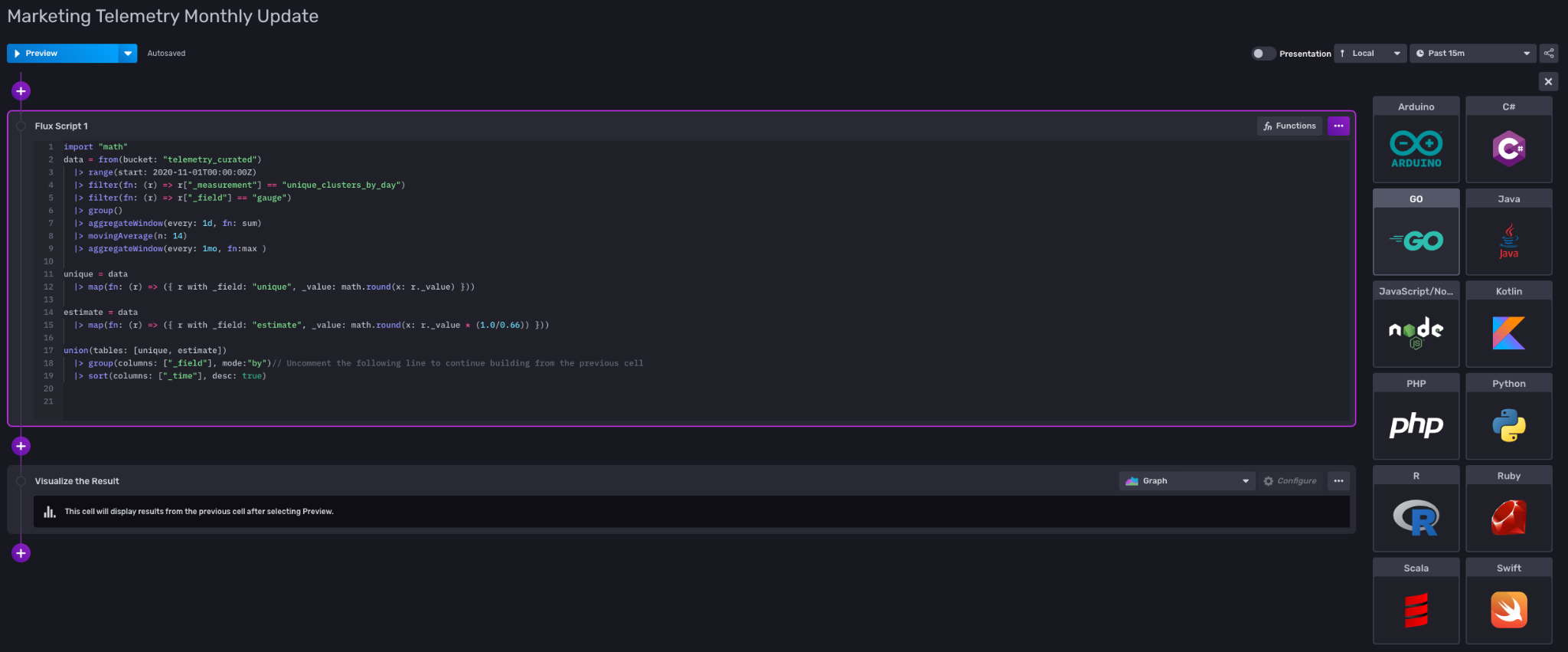
    The company has enhanced its InfluxDB Notebooks tool to enable developers to quickly set up an alert, build a task or write a Flux script without having to leave their browser.

    In addition, developers can compose Flux queries to be included in client code that can then be autogenerated within applications written in more than 10 different programming languages. There is now also an extension of Visual Studio Code that makes it simpler to create Flux scripts, query InfluxDB, create Flux tasks and manage buckets.

    Finally, InfluxData added the ability to explicitly define the schema of a bucket within InfluxDB to safeguard against unwanted changes; an application programming interface (API) tool, dubbed API Invocable Scripts, to make it simpler to define parameterized Flux scripts and the ability to send notifications from Alerta, WebEx Teams and ServiceNow to the InfluxDB Cloud platform.

    Tim Hall, vice president of product for InfluxData, said the overall goal is to reduce the level of complexity developers encounter when building applications that run on a time-series database. Many of those applications are now core to digital business transformation initiatives that require data to processed and analyzed over time. In effect, time-stamped data adds yet another dimension to any application, noted Hall.

    Time-series databases are typically employed by either an independent software vendor (ISV) to create, for example, a monitoring application, or an enterprise IT team that is building an application that lends itself to data that needs to be tracked over some period of time.

    In most instances, applications built on a time-series database are being deployed alongside, for example, relational databases that are generally invoked using SQL. As a result, InfluxDB has made it simpler to join data across relational and time-series data via SQL integrations the company added to Flux, noted Hall.

    DevOps teams, of course, are not always anxious to add another database they need to support, but as applications continue to evolve, more organizations are employing a mix of purpose-built databases to develop applications as the volume of data that organizations are trying to manage and analyze continues to grow.

    In the longer term, it’s clear time-series databases will play a critical role in driving digital business transformation initiatives. The challenge most organizations are now struggling with is determining which of these initiatives to prioritize. A time-series database coupled with the developer tools provided by InfluxData will enable IT teams to build the applications that drive those processes much faster, said Hall.

    In the meantime, IT teams would be well advised to at least become more familiar with time-series databases, because knowing the time when an event occurred is becoming a bigger application requirement. After all, knowing when something happened is now just as important as the record of what actually occurred.

  • How to Pivot and Join Time-Series Data in Flux

    How to Pivot and Join Time-Series Data in Flux

    Merging multiple time-series in InfluxDB using Flux may seem like a daunting task. This in-depth Flux tutorial will explain how to pivot, time shift and join time series in InfluxDB.

    In this InfluxDB tutorial, we will show you how to create an accurate overview of multiple time series with industrial data captured in consecutive production steps. Doing this requires a proper join mechanism for combining the time series into one after aligning them with respect to time.

    This tutorial is based on a real-world case we solved at Factry.io with InfluxDB in an industrial setting.

    Every second of the day, production sites all around the world are generating inconceivable amounts of process data. This data is directly acquired from production lines on-site and captured in the form of process parameters. Being able to reliably keep track of these process parameters throughout the production process is essential to continuously improving manufacturing operations.

    Industrial process parameters are represented as concurrent time series. They do not necessarily provide data points at a similar pace, nor are they always aligned over time. Obtaining a trustworthy overview of captured process parameters during consecutive production steps can be daunting.

    Time-Series Data Explained

    In brief, time-series data represents a number of different data points indexed by time. As time is a constituent of anything that is observable in our world, time-series data is everywhere. When narrowed down to a production environment, captured process parameters are distributed in time in order to become distinguishable from the process data preceding or following it.

    What is the difference between time-series and relational data? In contrast to time-series data, relational data holds records that are generally referenced by an artificial identifier. These identifiers can interrelate, which crafts the relational aspect.

    Pivot and Join Time-Series Data in Flux

    Before you get started

    On a production line, be aware that a product batch cannot be in two different production steps at the same point in time. As a result, time series measured in different production steps are naturally unaligned. Hence, before properly joining these time series into one, many of them will need to be shifted over time to get the overview right.

    Furthermore, retrieving data stored in a time-series database is commonly done by using the dedicated query language Flux.

    Two points about this:

    1. In Flux, a join can only make use of an inner join mechanism to melt multiple time series into one. As an inner join solely retains the data points for shared timestamps in multiple time series, data loss is unavoidable when dealing with unaligned time series or time series captured at different rates.
    2. In most use cases, only time series extracted from sensors at different production steps need to be joined. This is due to the ability to differentiate between multiple tables within one time series.

    Hence, reading in sensor data generated by multiple sensors at the same production step, table by table, allows us to bundle the sensor data. By ‘pivoting’ the tables into one, a time series is forged. Prior to being joined with the sensor data captured from another production step, the time series is shifted to align with respect to time. However, note that this requires all sensor data (potentially from different sensors) from one production step to be aggregated in the same way, omitting any differences in the rate at which it has been captured.

    Use Case: Welcome to the Cardboard Factory

    There are some best practices for pivoting and joining time series data in Flux from consecutive production steps. In this example, sensor data is captured from a replicated production site that is manufacturing cardboard panels out of recycled paperboard rolls.

    The production process of the cardboard factory consists of three different steps, which we’ll refer to as entries A, B and C.

    • In entry A, production starts with recycled paperboard rolls; the width and diameter of which is being measured by two separate sensors.
    • In entry B, the recycled paperboard rollsare cut into paperboard sheets and processed into cardboard using a certain temperature and pressure.
    • In entry C, the cardboard is cut into shape. For this entry, the height and the thickness of the panels are the key elements to be measured in terms of sensor data.

    With respect to time, it takes approximately one minute for the first sheet of recycled paperboard roll to reach entry B. Further, about two minutes elapse before the paperboard sheet is processed and shaped into a cardboard panel.

    Note that, in this production site, it is assumed that the speed of the production line is more or less fixed over time, making it possible to shift time series captured in different entries in order to get them aligned.

    Merging Multiple Time Series Into One Using Flux

    The goal in this use case is to create one trustworthy overview of all sensor data captured in each entry. Imagine today is May 4 at around 3:10 p.m. The overview should be reflecting all sensor data from the past ten minutes of the production site.

    Fortunately, we are aware that the sensor data between each entry is unaligned by a few minutes. Therefore, we should be fetching data between 3:00 and 3:10 with respect to the last entry (entry C); thereby trying to align these time series with the ones from both entry A and entry B.

    Think about it as being teleported to 3:10 on May 4. At that time, for a recycled paperboard roll in entry A or for a paperboard sheet in entry B, we do not yet have the sensor data for entry C. This is obviously because this sensor data will be captured only a few minutes later on the line.

    With this cleared up, a recycled paperboard roll delivered by one of the suppliers is referred to in the use case as a material lot. In contrast, a paperboard sheet derived from the recycled paperboard roll resulting in a cardboard panel is mentioned as a material sublot.

    At the end of the production line, a pile of cardboard panels is manufactured out of one material lot. To sum it up: In this use case, a material sublot can never be in two different entries at the same point in time, which means we need to align time series over consecutive entries.

    1. Reading in the Sensor Data

    First, we start by reading in the sensor data of both the width sensor and the diameter sensor for entry A. By reading in sensor data of both sensors in the same ‘filter’ (image: code snippet), we reduce this data to one time series for entry A.

    In this way, we hold different tables per sensor in one time series arranged by the group key consisting of ‘_field’ and ‘_measurement’. By reducing all sensor data from one entry to one time series holding multiple tables, the opportunity arises to pivot the tables into one unified table later on.

    Fetching the corresponding sensor data from entry A with respect to entry C is fulfilled by using a ‘range’ with sensor data that was captured between 2:57 and 3:07. This is applied by shifting the time range of entry A three minutes backward using ‘SHIFT_A’. Hence, for a cardboard panel at entry C, the corresponding sensor data at entry A was captured three minutes earlier.

    In essence, we are mapping the time range between 2:57 and 3:07 of entry A onto the time range between 3:00 and 3:10 of entry C and, thus, onto the overview.

    Note that for operations between a timestamp and a duration in ‘FROM_A’, you need to convert both the timestamp and the duration to an unsigned int to get Unix timestamps in ns prior to performing the calculation.

    Entry A sensor data – code snippet

    Entry A sensor data

    Regular and Irregular Time Series

    In most use cases, the sensor data will generate a regular time series (metrics), as the time period between captured data points will be fixed. However, when working with irregular time series (events) or time series generated at a different rate, these need to be transformed into a regular time series with an ‘aggregateWindow’ to eventually build up a nice overview.

    In this use case, there is only a regular time series. Therefore, retaining the ‘last’ data point for each time window of one minute should do the trick. In the case of an irregular time series, taking a ‘mean’ over a fixed time window would be the better choice.

    2. Pivoting the Time-Series Data

    After the sensor data from both sensors of entry A is collected into one time series with multiple tables, we now need to pivot the tables to become one. Therefore, the group key of each table needs to hold the same schema.

    In this use case, the group keys schema for all tables in the time series is as follows: ‘[‘_field’, ‘_measurement’]’. To make sure that the group keys schema is identical for all tables, we can use a ‘keep’ in front of the pivot to eliminate fields that are not present in all tables.

    Possible Deal-Breakers

    Bear in mind that the constraint for holding an identical schema for each table in the time series can be a deal-breaker for using the pivot. Another constraint lies in the lack of being able to pivot more than one value field, although when reading in sensor data from InfluxDB, there is typically only one value field.

    However, after adding some processing to the time series in Flux, chances are that an additional processed value column is present, eliminating the ability to use a pivot once more.

    When performing a pivot on multiple tables in the time series of entry A, for the table rows holding a shared timestamp (row key: ‘_time’), the data point in the value field (value column: ‘_value’) will be ingested into a column determined by the name of the measurement (column key: ‘_measurement’).

    In the use case, this means that the tables with the measurements ‘lot_ID’, ‘A_width’ and ‘A_diam’ will get their data points from the ‘_value’ field ingested into a separate column in the unified table, determined by their measurement names.

    In terms of performance, a pivot can suffer from having too many tables in the time series to be pivoted, which corresponds to the number of active sensors in one entry. Next to that, an extensive group key schema in the pivot will also take its toll. Having a considerable amount of rows per table in the time series of an entry with ns precision timestamps can easily blow up the pivot, as well.

    Finally, a small footnote on the functionality of the pivot in Flux. Keep in mind that the fields and tags that are not included in the pivot will not be ingested into the unified table. Additionally, the term pivot appears deceiving when being compared to its functionality in a relational database.

    Entry A pivot – code snippet

    Entry A shift


    3. Time Shifting the Time Series Data

    Entry A

    After pivoting the sensor data of entry A into one unified table, the entry A sensor data with time range between 2:57 and 3:07 gets aligned with the time range of the overview between 15:00 and 15:10 by performing a time shift of three minutes forward on the _time column.

    To preserve the original timestamps of entry A, we take a duplicate of the _time column in the unified table and refer to it as the time for which a sublot actually started at entry A, mentioned as entry_A.

    entry A shifted – code snippet

    Entry A Shift – Code Snippet

    Entry A Shift

    Entry B & C

    The same procedure for reading in the sensor data of entry A applies for entry B and entry C. While the sensor data for the former is shifted by two minutes to get its time range between 2:58 and 3:08 aligned with the time range of the overview, the sensor data of the latter is already in sync for the overview.

    Entry B – code snippet


    Entry B

    Entry C – code snippet


    Entry C


    4a. Joining the Time Series

    After pivoting the sensor data for each entry, three distinct time series are held, each containing one table with a separate schema and multiple value columns; for example, ‘C_height’ and ‘C_thickness’ for entry C. To create one overview, these three time series must be joined together, visualizing the data points of different sensors side-by-side with respect to time. Since the sensor data of the different entries has been formerly aligned by reading in the corresponding time ranges for each entry followed by a ‘timeshift’, the three time series can now be joined on the synced ‘_time’ column present in each of them.

    Possible Issues

    Since the schema differs between the three time series tables, you would encounter significant overhead when trying to pivot these three tables into one after appending them to a single new time series. Besides the superfluous complexity added, the tables of all time series are each holding more than one value column, which makes the pivot unusable in this case.

    A plausible solution would be to use a ‘join’ provided by Flux on the aligned ‘_time’ column. As discussed in the pivot and join section, the ‘join’ is represented as an inner join mechanism, solely retaining data points for shared timestamps between joined tables.

    In this use case, the inner join mechanism would not trigger any data loss, since only regular and aligned time series are present after the pivot. However in case of irregular time series (not using ‘aggregateWindow’ on events), time series captured at a different rate or regular yet unaligned time series, data points would get lost in the inner join mechanism.

    Next to that, the ‘join’ in Flux is only letting two time series be joined together at once, which constrains the possibilities. Moreover, seen from a performance perspective, the ‘join’ is considerably less optimized compared to dedicated functions in Flux, like the ‘aggregateWindow’.

    4b. Solution: Outer Join

    To tackle the issues subject to the ‘join’ provided by Flux, an outer join mechanism is proposed, retaining data points for both shared and unshared timestamps between tables of multiple joined time series with respect to time. After appending the three time series to a single new time series holding one table, the outer join mechanism groups all data points by time into ‘timetables’ prior to filling up rows with the appropriate data points. Furthermore, the single complete row per timetable is extracted, preceding the ungrouping of timetables to one overview table.

    Union

    Once the aligned sensor data is available into a dedicated time series per entry consisting of one table, the three time series are appended by a ‘union’ to a single new time series holding one table. The ‘union’ is ingesting the sensor data of each entry vertically (image: union), meaning the table rows per entry are placed underneath each other while the resulting table schema is the union of the separate table schemas of the three time series. In this manner, you can witness ‘data point blocks’ in the resulting table referring to sensor data of each entry in the production site. Note that the ‘union’ allows more than two time series to be appended to a new single time series at once.

    union – code snippet

    union


    Timetables

    The sensor data of all three entries in the single time series table is grouped by the ‘_time’ column to group the sensor data of different entries together in timetables. The ‘timetables’ refer to the tables that arise by using the group key ‘_time’ (image timetables). The forthcoming sort is fundamental to order the rows of a certain entry at the bottom of a timetable prior to starting to fill data points. In this use case the row originating from entry C is positioned at the bottom of each timetable’ by sorting for the ‘entry_C’ column in ascending order. In fact, regardless of sorting the ‘entry_C’ column in ascending or descending order, the empty data points in the ‘entry_C’ column of the rows originating from entry A or entry B will always be on top in Flux since they hold a null value.

    Timetables – code snippet

    Timetables 

    Fill

    Moving forward, the data points of the columns originating from entry A and entry B are copied into subsequent rows using the ‘fill’ with ‘usePrevious’ set to ‘true’. Since the data points are filled through the bottom, the mutual order of the rows originating from entry A and entry B is not important. Note that at the bottom of each timetable, the row originating from entry C is now a complete row holding all data points for all three entries (image: fill).

    fill – code snippet 

    fill

    Extract

    Finally, only the complete row at the bottom of each timetable is extracted by using the ‘tail’ with ‘n’ set to ‘1’. The timetables are ungrouped to one joined table by using the ‘group’ without any parameters to empty the group key. Check out the joined table (image: extract) and you’ll see that all sensor data originating from the three entries of the production site is visualized into one trustworthy overview with respect to the time behavior induced by a sublot passing through the production entries on site.

    Extract – code snippet 

    Extract


    4c. Outer Join Mechanism for Unaligned Sensor Data

    To illustrate the outer join mechanism, one can join unaligned sensor data for the corresponding time ranges from the 3 entries in the production site into one overview. This can be arranged by removing both the ‘timeShift’ of three minutes for entry A and the ‘timeShift’ of two minutes for entry B when compared to entry C.

    In that case, the sensor data of entry A will retain its time range between 2:57 and 3:07, while entry B will have a time range between 2:58 and 3:08, followed by a time range between 3:00 and 3:10 for entry C. The result is a broader overall time range for the overview than requested (image: outer join on unshifted sensor data). Besides, only unaligned sensor data is present for all three entries in the time range between 3:00 and 3:07.

    Note that for the top and the bottom rows, the unavailable sensor data for a certain entry is replaced by the ingestion of null values as data points in the columns are originating from the corresponding entry. As mentioned earlier, the same principles apply for an outer join when dealing with irregular time series or time series captured at a different rate. Ideally, such an outer join mechanism should be the default behavior in Flux when performing a ‘join’.

    Outer join on unshifted sensor data 

    Conclusion

    When creating a trustworthy overview of captured sensor data at a production site in consecutive production steps, take these four elements into account:

    1. The step in the production process where the sensor data is captured is key to understanding the time behavior of a product batch going through the different production steps on site.
    2. How sensor data is captured in production indicates the urgency of using a specific time window and which selection/aggregation of data points you should obtain. Hence, sensor data can generate a regular or irregular time series or can be captured at a different rate.
    3. Sensor data per production step is pivoted to a time series holding one unified table of sensor data for that production step. The pivot stands out in unifying the sensor data per production step, since the different tables each referencing a sensor in that production step typically hold an identical schema when reading them in.
      • Next to that, generally speaking, there will only be one data stream per sensor and thus only one value field per table in the time series derived from a production step.
      • Performing an outer join on the multiple time series originating from multiple production steps, gives you the ability to create a trustworthy overview in the end. To make the most out of it, make sure to align the time series first before joining them.
  • Time Series Virtual Summit Speaker Spotlight: Jon Herlocker and Miroslav Malecha

    Time Series Virtual Summit Speaker Spotlight: Jon Herlocker and Miroslav Malecha

    The Time Series Virtual Summit will bring together InfluxData community members for a unique learning experience focused on the impact of time series data. Presented in a virtual reality environment, the event will take place on July 16, at 10 a.m. EDT.

    Miroslav Malecha
    Jon Herlocker

    Jon Herlocker, president and CEO at Tignis, is one of the speakers that will be presenting at the Time Series Virtual Summit.

    Jon invites anybody who has the responsibility to turn large quantities of sensor data from physical plants or manufacturing lines into business value to attend his session, “How an Analytics Platform Detects Reliability Threats and Eliminates Obstacles Impeding Results Using InfluxDB.”

    “Viewers will see Tignis’ unique physics-driven approach to machine learning for physical plants and manufacturing lines,” said Jon. “We’ll also share our approach to using InfluxDB to accelerate delivery of our solution to our customers.”

    Jon will discuss how Tignis uses IoT sensors to reduce unexpected downtime at manufacturing plants and school campuses. Attendees will learn how by using a time series database they can improve their competitive advantage and accelerate their go-to-market strategy.

    “Time series data from physical plants and manufacturing lines can be turned into significant business value, and we have proven that InfluxDB can be an effective component of that,” said Jon.

    Another time series specialist that will be sharing his knowledge and his experience with InfluxDB is Miroslav Malecha, director of product management at Bonitoo.

    In his session, “Using Time Series for Geo-Temporal Analysis,” Miroslav will discuss how to use InfluxDB’s Flux for Geo-Temporal analysis. He’ll briefly cover what Flux is, how to use specific Flux geo functions and finish with a quick demo of how to use InfluxDB.

    You can hear from Jon, Miroslav and more time series experts at the Time Series Virtual Summit. To check out the agenda, the full lineup of speakers and to register (for free), visit the Time Series Virtual Summit website.

  • Time Series Virtual Summit Speaker Spotlight: Al Sargent and Samantha Wang

    Time Series Virtual Summit Speaker Spotlight: Al Sargent and Samantha Wang

    The Time Series Virtual Summit will bring together InfluxData community members for a unique learning experience focused on the impact of time series data. Presented in a virtual reality environment, the event will take place on July 16, at 10 a.m. EDT.

    Samantha Wang
    Al Sargent

    Al Sargent and Samantha Wang of InfluxData are on a mission to help developers understand how time series databases provide real-time observability and monitoring.

    “The best software engineering teams in the world understand that time series data is different; it can’t be managed using a traditional database, and requires a purpose-built database,” said Al Sargent, senior director of product marketing at InfluxData.

    Al will be the first speaker to take the virtual stage at the Time Series Virtual Summit. During his presentation, he will explore the unique challenges of managing time-series data, why time series data needs to be treated differently than other data types and what to look for in a time series database.

    Any developer that’s building applications using time series data (or planning to), such as data from IoT sensors, monitoring data or customer usage data will benefit from Al’s educational session.

    Another great session you must definitely attend is “Monitor your Cloud Metrics with Time Series” by Samantha Wang, product manager at InfluxData.

    Samantha will discuss the importance of time series data for cloud monitoring, and how you can view your metrics in real time with InfluxDB Cloud.

    “I will walk through how to write metrics into InfluxDB Cloud using Telegraf and how users can take their analysis one step further with Flux,” said Samantha. “Lastly, I will review InfluxDB Templates, one of our newest community InfluxDB products, that provides a packaged solution for various common monitoring use cases.”

    Join Al and Samantha to learn more about time series databases and understand how InfluxDB Cloud can be your end-to-end solution for writing data to monitoring and alerting — all optimized for time series data.

    You can hear from Al, Samantha and more time series experts at the Time Series Virtual Summit. To check out the agenda, the full lineup of speakers and to register (for free), visit the Time Series Virtual Summit website.

  • Time Series Virtual Summit Speaker Spotlight: John Gleeson and Benjamin Sirb

    Time Series Virtual Summit Speaker Spotlight: John Gleeson and Benjamin Sirb

    The Time Series Virtual Summit will bring together InfluxData community members for a unique learning experience focused on the impact of time series data. Presented in a virtual reality environment, the event will take place on July 16, at 10 a.m. EDT.

    Benjamin Sirb
    John Gleeson

    John Gleeson and Benjamin Sirb of Storj Labs, will be at the Time Series Virtual Summit to discuss how the InfluxDB contributes to Stroj’s decentralized cloud storage platform.

    “Our team uses time series data to operate our decentralized cloud storage platform, which provides enterprise-grade object storage and is the largest of its kind,” said John Gleeson, vice president of operations at Storj Labs.

    Tardigrade, powered by Storj Labs, offers decentralized cloud storage that is automatically encrypted, easily implemented, highly performant, very economical and resilient. By equipping their customers with fast, secure and fully distributed storage, their users no longer need to manage their infrastructure. The Storj platform enables applications to store and share data across a distributed network with end-to-end encryption.

    In their talk, John and Ben will dive into:

    • Storj’s redefinition of a cloud object storage network.
    • How InfluxData fits into Storj’s Open Source Partner Program.
    • Collecting and managing high volume real-time telemetry data from a distributed network.

    “Attendees can expect a deep dive on how time series data allows for real-time analysis of a highly complex system, which operates in a low trust environment while maintaining industry standard SLA’s for data availability and durability,” said Benjamin Sirb, senior data scientist at Storj Labs.

    As vice president of operations, John is responsible for direct sales, partnerships, customer success, community, product management and data science as well as growing the international presence for the Storj decentralized and distributed cloud storage network. He is responsible for operationalizing core processes to ensure the business scales as the company and network grow.

    Ben joined Storj Labs in 2018, bringing six years of experience in academia, research and consulting to his role as senior data scientist. Drawing from his knowledge of probability theory, Ben has been instrumental in researching the theoretical foundations and practical applications of decentralized networks at Storj.

    If there is one thing they both would like the audience to keep in mind is that “the data science behind distributed and decentralized cloud storage is intense!”

    Join John and Ben to discover how InfluxDB is a component to Storj’s Tardigrade service and workflows.

    You can hear from Ben, John and more time series experts at the Time Series Virtual Summit. To check out the agenda, the full lineup of speakers and to register (for free), visit the Time Series Virtual Summit website.

  • Time Series Virtual Summit Speaker Spotlight: James Governor, Sameer Farooqui and Russ Savage

    Time Series Virtual Summit Speaker Spotlight: James Governor, Sameer Farooqui and Russ Savage

    The Time Series Virtual Summit will bring together InfluxData community members for a unique learning experience focused on the impact of time series data. Presented in a virtual reality environment, the event will take place on July 16, at 10 a.m. EDT.


    Russ Savage
    Russ Savage
    Sameer Farooqui
    Sameer Farooqui
    James Governor
    James Governor

    The Time Series Virtual Summit features a stellar lineup of time series experts, including Sameer Farooqui, Russ Savage and keynote speaker James Governor.

    James Governor is an analyst and co-founder at RedMonk. James advises developers on technology strategies, open source and how to be more productive. During his keynote presentation, “Reframing and Retooling for Observability,” he will explain how observability is changing the way applications are built and managed. James will also discuss what this means for developers and how observability can be used to derive deep insights into system performance and user experience.

    Sameer Farooqui is a strategic cloud engineer at Google. Sameer focuses on Streaming Analytics and helps commercialize new streaming solutions such as time series forecasting and anomaly detection. In his session, “Analytics and ML on Time Series Data in Google Cloud,” Sameer will talk about the benefits of running time series databases in the Google Cloud Platform, and how to take advantage of Google Analytics tools.

    Russ Savage is a product manager at InfluxData, where he focuses on enabling DevOps for teams using InfluxDB and the TICK Stack. Russ will give the closing remarks, wrapping up the event with ways to get involved and learn more about the time series community.

    You can hear from James, Sameer, Russ and more time series experts at the Time Series Virtual Summit. To check out the agenda, the full lineup of speakers and to register (for free), visit the Time Series Virtual Summit website.

  • Upcoming Event: Time Series Virtual Summit

    Upcoming Event: Time Series Virtual Summit

    The Time Series Virtual Summit will bring together InfluxData community members for a unique learning experience focused on the impact of time series data. Presented in a virtual reality environment, the event will take place on July 16, from 10 a.m. to 4 p.m. EDT.

    This virtual event will focus on the impact of time series data and how it can be used to help build and optimize solutions for real-time visibility into stacks, sensors and systems.

    Here’s a preview of some of the speakers:

    • James Governor, analyst and co-founder at RedMonk
    • Al Sargent, senior director of product marketing at InfluxData
    • John Gleeson, VP of operations at Tardigrade.io
    • Jon Herlocker, president and CEO at Tignis
    • Michael Ellis, community manager at InfluxData

    Plus, speakers from companies such as AWS, Google, Microsoft and more.

    The industry leaders will share their thoughts on time series data, discuss the benefits of a time series database and the challenges of data management.

    At the Time Series Virtual Summit you will learn:

    • How to use a time series database to improve their competitive advantage and accelerate their go-to-market strategy.
    • How to manage risk in decentralized networks with time series.
    • How IoT can help manufacturers reduce downtime.
    • How to use observability to derive deep insights into system performance and user experience.

    The online environment features a lobby, an expo hall lined with booths full of downloadable resources, and an auditorium where attendees can watch the sessions. You can interact directly with time series experts and network with other attendees by joining the chat rooms.

    Discover what’s next from the InfluxData community and learn how you can get involved. To check out the agenda, the full lineup of speakers and to register (for free), visit the Time Series Virtual Summit website.