Tag: database

  • Verica Launches Database for Sharing IT Incident Reports

    Verica Launches Database for Sharing IT Incident Reports

    Verica, a provider of an incident management platform, announced this week it is making available a database to make incident reports publicly available via a single repository.

    Courtney Nash, senior research analyst at Verica, said the Verica Open Incident Database (VOID) initiative is part of an effort to enable organizations to learn from outages and failures caused by software. Today, reports about such incidents tend to be difficult to find because they are scattered all across the internet, she added.

    That lack of transparency makes it difficult to compare and contrast incidents in a way that surfaces meaningful insights, noted Nash.

    Launch partners for the VOID include Indeed, NS1, Adaptive Capacity Labs, Security Scorecard and Auxon. Each will provide support to help fund the development, research and dissemination of knowledge generated by the project.

    The VOID contains more than just standard company postmortems or status updates, added Nash. Verica is committed to applying metadata to better understand how individuals, companies, media and others reacted during an incident.

    One early finding already derived from this initiative is that mean-time-to-resolve (MTTR) is proving to be an inaccurate metric due to the varied distribution of incident data. Other findings include the fact that only one-quarter of incident reports took the time to identify the root cause of an issue, while less than 1% took the time to study incident reports of near-misses.

    In general, there’s now more riding on the performance and availability of IT environments than ever. Digital business transformation became all the rage in the wake of the economic downturn brought on by the COVD-19 pandemic. As the economy continues to recover, businesses now expect IT to respond and pivot to changing conditions no matter how sudden.

    DevOps teams have, of course, learned to expect the unexpected by embracing modern incident management based on DevOps best practices that enable IT teams to adroitly respond to any outage or sudden degradation in application performance. The most important thing to remember about incident management is that practice makes perfect. While practice runs may never precisely mirror an actual crisis, organizations that have processes that are well-known by their IT incident teams and that practice ‘fire drills’ tend to respond both faster and better. After all, the more muscle memory there is to call on the more resilient the organization will be.

    It’s not clear to what degree IT organizations will be willing to share incident reports. However, there is an opportunity for IT professionals to come together that is similar to how engineers from different airlines collaborated to make flying safer for the general public, said Nash. In fact, with so many processes now dependent on software, it’s amazing there have not been more catastrophic events due to software issues. It’s even arguable that it’s only a matter of time before such levels of collaboration are mandated.

    In the meantime, the first step toward achieving that goal may simply be sharing a report with colleagues so they can learn from previous mistakes.

  • How to Pivot and Join Time-Series Data in Flux

    How to Pivot and Join Time-Series Data in Flux

    Merging multiple time-series in InfluxDB using Flux may seem like a daunting task. This in-depth Flux tutorial will explain how to pivot, time shift and join time series in InfluxDB.

    In this InfluxDB tutorial, we will show you how to create an accurate overview of multiple time series with industrial data captured in consecutive production steps. Doing this requires a proper join mechanism for combining the time series into one after aligning them with respect to time.

    This tutorial is based on a real-world case we solved at Factry.io with InfluxDB in an industrial setting.

    Every second of the day, production sites all around the world are generating inconceivable amounts of process data. This data is directly acquired from production lines on-site and captured in the form of process parameters. Being able to reliably keep track of these process parameters throughout the production process is essential to continuously improving manufacturing operations.

    Industrial process parameters are represented as concurrent time series. They do not necessarily provide data points at a similar pace, nor are they always aligned over time. Obtaining a trustworthy overview of captured process parameters during consecutive production steps can be daunting.

    Time-Series Data Explained

    In brief, time-series data represents a number of different data points indexed by time. As time is a constituent of anything that is observable in our world, time-series data is everywhere. When narrowed down to a production environment, captured process parameters are distributed in time in order to become distinguishable from the process data preceding or following it.

    What is the difference between time-series and relational data? In contrast to time-series data, relational data holds records that are generally referenced by an artificial identifier. These identifiers can interrelate, which crafts the relational aspect.

    Pivot and Join Time-Series Data in Flux

    Before you get started

    On a production line, be aware that a product batch cannot be in two different production steps at the same point in time. As a result, time series measured in different production steps are naturally unaligned. Hence, before properly joining these time series into one, many of them will need to be shifted over time to get the overview right.

    Furthermore, retrieving data stored in a time-series database is commonly done by using the dedicated query language Flux.

    Two points about this:

    1. In Flux, a join can only make use of an inner join mechanism to melt multiple time series into one. As an inner join solely retains the data points for shared timestamps in multiple time series, data loss is unavoidable when dealing with unaligned time series or time series captured at different rates.
    2. In most use cases, only time series extracted from sensors at different production steps need to be joined. This is due to the ability to differentiate between multiple tables within one time series.

    Hence, reading in sensor data generated by multiple sensors at the same production step, table by table, allows us to bundle the sensor data. By ‘pivoting’ the tables into one, a time series is forged. Prior to being joined with the sensor data captured from another production step, the time series is shifted to align with respect to time. However, note that this requires all sensor data (potentially from different sensors) from one production step to be aggregated in the same way, omitting any differences in the rate at which it has been captured.

    Use Case: Welcome to the Cardboard Factory

    There are some best practices for pivoting and joining time series data in Flux from consecutive production steps. In this example, sensor data is captured from a replicated production site that is manufacturing cardboard panels out of recycled paperboard rolls.

    The production process of the cardboard factory consists of three different steps, which we’ll refer to as entries A, B and C.

    • In entry A, production starts with recycled paperboard rolls; the width and diameter of which is being measured by two separate sensors.
    • In entry B, the recycled paperboard rollsare cut into paperboard sheets and processed into cardboard using a certain temperature and pressure.
    • In entry C, the cardboard is cut into shape. For this entry, the height and the thickness of the panels are the key elements to be measured in terms of sensor data.

    With respect to time, it takes approximately one minute for the first sheet of recycled paperboard roll to reach entry B. Further, about two minutes elapse before the paperboard sheet is processed and shaped into a cardboard panel.

    Note that, in this production site, it is assumed that the speed of the production line is more or less fixed over time, making it possible to shift time series captured in different entries in order to get them aligned.

    Merging Multiple Time Series Into One Using Flux

    The goal in this use case is to create one trustworthy overview of all sensor data captured in each entry. Imagine today is May 4 at around 3:10 p.m. The overview should be reflecting all sensor data from the past ten minutes of the production site.

    Fortunately, we are aware that the sensor data between each entry is unaligned by a few minutes. Therefore, we should be fetching data between 3:00 and 3:10 with respect to the last entry (entry C); thereby trying to align these time series with the ones from both entry A and entry B.

    Think about it as being teleported to 3:10 on May 4. At that time, for a recycled paperboard roll in entry A or for a paperboard sheet in entry B, we do not yet have the sensor data for entry C. This is obviously because this sensor data will be captured only a few minutes later on the line.

    With this cleared up, a recycled paperboard roll delivered by one of the suppliers is referred to in the use case as a material lot. In contrast, a paperboard sheet derived from the recycled paperboard roll resulting in a cardboard panel is mentioned as a material sublot.

    At the end of the production line, a pile of cardboard panels is manufactured out of one material lot. To sum it up: In this use case, a material sublot can never be in two different entries at the same point in time, which means we need to align time series over consecutive entries.

    1. Reading in the Sensor Data

    First, we start by reading in the sensor data of both the width sensor and the diameter sensor for entry A. By reading in sensor data of both sensors in the same ‘filter’ (image: code snippet), we reduce this data to one time series for entry A.

    In this way, we hold different tables per sensor in one time series arranged by the group key consisting of ‘_field’ and ‘_measurement’. By reducing all sensor data from one entry to one time series holding multiple tables, the opportunity arises to pivot the tables into one unified table later on.

    Fetching the corresponding sensor data from entry A with respect to entry C is fulfilled by using a ‘range’ with sensor data that was captured between 2:57 and 3:07. This is applied by shifting the time range of entry A three minutes backward using ‘SHIFT_A’. Hence, for a cardboard panel at entry C, the corresponding sensor data at entry A was captured three minutes earlier.

    In essence, we are mapping the time range between 2:57 and 3:07 of entry A onto the time range between 3:00 and 3:10 of entry C and, thus, onto the overview.

    Note that for operations between a timestamp and a duration in ‘FROM_A’, you need to convert both the timestamp and the duration to an unsigned int to get Unix timestamps in ns prior to performing the calculation.

    Entry A sensor data – code snippet

    Entry A sensor data

    Regular and Irregular Time Series

    In most use cases, the sensor data will generate a regular time series (metrics), as the time period between captured data points will be fixed. However, when working with irregular time series (events) or time series generated at a different rate, these need to be transformed into a regular time series with an ‘aggregateWindow’ to eventually build up a nice overview.

    In this use case, there is only a regular time series. Therefore, retaining the ‘last’ data point for each time window of one minute should do the trick. In the case of an irregular time series, taking a ‘mean’ over a fixed time window would be the better choice.

    2. Pivoting the Time-Series Data

    After the sensor data from both sensors of entry A is collected into one time series with multiple tables, we now need to pivot the tables to become one. Therefore, the group key of each table needs to hold the same schema.

    In this use case, the group keys schema for all tables in the time series is as follows: ‘[‘_field’, ‘_measurement’]’. To make sure that the group keys schema is identical for all tables, we can use a ‘keep’ in front of the pivot to eliminate fields that are not present in all tables.

    Possible Deal-Breakers

    Bear in mind that the constraint for holding an identical schema for each table in the time series can be a deal-breaker for using the pivot. Another constraint lies in the lack of being able to pivot more than one value field, although when reading in sensor data from InfluxDB, there is typically only one value field.

    However, after adding some processing to the time series in Flux, chances are that an additional processed value column is present, eliminating the ability to use a pivot once more.

    When performing a pivot on multiple tables in the time series of entry A, for the table rows holding a shared timestamp (row key: ‘_time’), the data point in the value field (value column: ‘_value’) will be ingested into a column determined by the name of the measurement (column key: ‘_measurement’).

    In the use case, this means that the tables with the measurements ‘lot_ID’, ‘A_width’ and ‘A_diam’ will get their data points from the ‘_value’ field ingested into a separate column in the unified table, determined by their measurement names.

    In terms of performance, a pivot can suffer from having too many tables in the time series to be pivoted, which corresponds to the number of active sensors in one entry. Next to that, an extensive group key schema in the pivot will also take its toll. Having a considerable amount of rows per table in the time series of an entry with ns precision timestamps can easily blow up the pivot, as well.

    Finally, a small footnote on the functionality of the pivot in Flux. Keep in mind that the fields and tags that are not included in the pivot will not be ingested into the unified table. Additionally, the term pivot appears deceiving when being compared to its functionality in a relational database.

    Entry A pivot – code snippet

    Entry A shift


    3. Time Shifting the Time Series Data

    Entry A

    After pivoting the sensor data of entry A into one unified table, the entry A sensor data with time range between 2:57 and 3:07 gets aligned with the time range of the overview between 15:00 and 15:10 by performing a time shift of three minutes forward on the _time column.

    To preserve the original timestamps of entry A, we take a duplicate of the _time column in the unified table and refer to it as the time for which a sublot actually started at entry A, mentioned as entry_A.

    entry A shifted – code snippet

    Entry A Shift – Code Snippet

    Entry A Shift

    Entry B & C

    The same procedure for reading in the sensor data of entry A applies for entry B and entry C. While the sensor data for the former is shifted by two minutes to get its time range between 2:58 and 3:08 aligned with the time range of the overview, the sensor data of the latter is already in sync for the overview.

    Entry B – code snippet


    Entry B

    Entry C – code snippet


    Entry C


    4a. Joining the Time Series

    After pivoting the sensor data for each entry, three distinct time series are held, each containing one table with a separate schema and multiple value columns; for example, ‘C_height’ and ‘C_thickness’ for entry C. To create one overview, these three time series must be joined together, visualizing the data points of different sensors side-by-side with respect to time. Since the sensor data of the different entries has been formerly aligned by reading in the corresponding time ranges for each entry followed by a ‘timeshift’, the three time series can now be joined on the synced ‘_time’ column present in each of them.

    Possible Issues

    Since the schema differs between the three time series tables, you would encounter significant overhead when trying to pivot these three tables into one after appending them to a single new time series. Besides the superfluous complexity added, the tables of all time series are each holding more than one value column, which makes the pivot unusable in this case.

    A plausible solution would be to use a ‘join’ provided by Flux on the aligned ‘_time’ column. As discussed in the pivot and join section, the ‘join’ is represented as an inner join mechanism, solely retaining data points for shared timestamps between joined tables.

    In this use case, the inner join mechanism would not trigger any data loss, since only regular and aligned time series are present after the pivot. However in case of irregular time series (not using ‘aggregateWindow’ on events), time series captured at a different rate or regular yet unaligned time series, data points would get lost in the inner join mechanism.

    Next to that, the ‘join’ in Flux is only letting two time series be joined together at once, which constrains the possibilities. Moreover, seen from a performance perspective, the ‘join’ is considerably less optimized compared to dedicated functions in Flux, like the ‘aggregateWindow’.

    4b. Solution: Outer Join

    To tackle the issues subject to the ‘join’ provided by Flux, an outer join mechanism is proposed, retaining data points for both shared and unshared timestamps between tables of multiple joined time series with respect to time. After appending the three time series to a single new time series holding one table, the outer join mechanism groups all data points by time into ‘timetables’ prior to filling up rows with the appropriate data points. Furthermore, the single complete row per timetable is extracted, preceding the ungrouping of timetables to one overview table.

    Union

    Once the aligned sensor data is available into a dedicated time series per entry consisting of one table, the three time series are appended by a ‘union’ to a single new time series holding one table. The ‘union’ is ingesting the sensor data of each entry vertically (image: union), meaning the table rows per entry are placed underneath each other while the resulting table schema is the union of the separate table schemas of the three time series. In this manner, you can witness ‘data point blocks’ in the resulting table referring to sensor data of each entry in the production site. Note that the ‘union’ allows more than two time series to be appended to a new single time series at once.

    union – code snippet

    union


    Timetables

    The sensor data of all three entries in the single time series table is grouped by the ‘_time’ column to group the sensor data of different entries together in timetables. The ‘timetables’ refer to the tables that arise by using the group key ‘_time’ (image timetables). The forthcoming sort is fundamental to order the rows of a certain entry at the bottom of a timetable prior to starting to fill data points. In this use case the row originating from entry C is positioned at the bottom of each timetable’ by sorting for the ‘entry_C’ column in ascending order. In fact, regardless of sorting the ‘entry_C’ column in ascending or descending order, the empty data points in the ‘entry_C’ column of the rows originating from entry A or entry B will always be on top in Flux since they hold a null value.

    Timetables – code snippet

    Timetables 

    Fill

    Moving forward, the data points of the columns originating from entry A and entry B are copied into subsequent rows using the ‘fill’ with ‘usePrevious’ set to ‘true’. Since the data points are filled through the bottom, the mutual order of the rows originating from entry A and entry B is not important. Note that at the bottom of each timetable, the row originating from entry C is now a complete row holding all data points for all three entries (image: fill).

    fill – code snippet 

    fill

    Extract

    Finally, only the complete row at the bottom of each timetable is extracted by using the ‘tail’ with ‘n’ set to ‘1’. The timetables are ungrouped to one joined table by using the ‘group’ without any parameters to empty the group key. Check out the joined table (image: extract) and you’ll see that all sensor data originating from the three entries of the production site is visualized into one trustworthy overview with respect to the time behavior induced by a sublot passing through the production entries on site.

    Extract – code snippet 

    Extract


    4c. Outer Join Mechanism for Unaligned Sensor Data

    To illustrate the outer join mechanism, one can join unaligned sensor data for the corresponding time ranges from the 3 entries in the production site into one overview. This can be arranged by removing both the ‘timeShift’ of three minutes for entry A and the ‘timeShift’ of two minutes for entry B when compared to entry C.

    In that case, the sensor data of entry A will retain its time range between 2:57 and 3:07, while entry B will have a time range between 2:58 and 3:08, followed by a time range between 3:00 and 3:10 for entry C. The result is a broader overall time range for the overview than requested (image: outer join on unshifted sensor data). Besides, only unaligned sensor data is present for all three entries in the time range between 3:00 and 3:07.

    Note that for the top and the bottom rows, the unavailable sensor data for a certain entry is replaced by the ingestion of null values as data points in the columns are originating from the corresponding entry. As mentioned earlier, the same principles apply for an outer join when dealing with irregular time series or time series captured at a different rate. Ideally, such an outer join mechanism should be the default behavior in Flux when performing a ‘join’.

    Outer join on unshifted sensor data 

    Conclusion

    When creating a trustworthy overview of captured sensor data at a production site in consecutive production steps, take these four elements into account:

    1. The step in the production process where the sensor data is captured is key to understanding the time behavior of a product batch going through the different production steps on site.
    2. How sensor data is captured in production indicates the urgency of using a specific time window and which selection/aggregation of data points you should obtain. Hence, sensor data can generate a regular or irregular time series or can be captured at a different rate.
    3. Sensor data per production step is pivoted to a time series holding one unified table of sensor data for that production step. The pivot stands out in unifying the sensor data per production step, since the different tables each referencing a sensor in that production step typically hold an identical schema when reading them in.
      • Next to that, generally speaking, there will only be one data stream per sensor and thus only one value field per table in the time series derived from a production step.
      • Performing an outer join on the multiple time series originating from multiple production steps, gives you the ability to create a trustworthy overview in the end. To make the most out of it, make sure to align the time series first before joining them.
  • Achieving Business Maturity with Database DevOps

    Achieving Business Maturity with Database DevOps

    Companies have seen unprecedented change over the past year and a half, with IT teams trying to help businesses weather the storm by meeting customer demands for services and products to be delivered in new ways while adjusting to remote work. As more companies introduced hybrid approaches to their workplace, a particular trend began to emerge: DevOps adoption. 

    Many adopted DevOps to navigate the new landscape, boosting software delivery and operational performance with advanced application and database development practices. In fact, research from Redgate Software indicates that DevOps adoption reached its peak earlier this year, with 26% of enterprises leveraging DevOps across all projects—a significant increase from previous adoption rates.

    Although not all companies have been quick to adopt for fear of disrupting existing workflows, a technical skills gap or lack of buy-in from management, there is a strong case to be made for why adopting DevOps practices, including for the database, can help businesses better manage the evolving tech environment.

    Adopting Automated Deployments

    Companies everywhere migrated databases to the cloud over the course of the past year, and that trend shows no sign of slowing. Analysts at IDC predict that by 2022 more than 90% of enterprises will rely on a mixture of on-premises/dedicated private clouds, multiple public clouds and legacy platforms to meet their needs. One of the best ways to help maintain that data is to implement DevOps processes for those databases and automate deployments. This provides a host of benefits, including: 

    • Preventing software errors: Manual database migrations often come with a host of errors that lead to downtime, rollbacks and rework. It’s far better to rely on an automated process that is robust and repeatable and can be implemented across all databases to ensure they’re updated in the same, reliable way. 
    • Staying in the loop: Knowledge of how to release updates and changes is often limited to a handful of people or even just one person. If, instead, it is part of the system and development process, it ensures everyone is in sync with updates and developments and allows anyone on your IT team to handle deployments.
    • Guaranteeing quality and consistency: For companies with security and compliance concerns, the predictable and repeatable processes that automated database deployments introduce ensure nothing is left to chance, while providing an auditable record of exactly what was changed, when and by who.

    Although the research shows 20% of companies cite cost as a roadblock to automation, avoiding automation will leave businesses at a disadvantage as they prepare for the coming year. 

    Creating Communities of Practice 

    When asked how they decide the strategic direction and planning for DevOps, the most popular answer from respondents was communities of practice. This concept was proposed for the first time in the early 1990s, and the practice has seen increased popularity among IT teams recently. It’s described as groups of people who share the same passions or concerns for something they do and often learn how to do that task better based on their regular, frequent interactions. 

    These various communities—regardless of whether in-person or virtual, given the current environment—help foster intrinsic motivation in employees and improve overall decision-making and encourage innovation. According to Redgate’s research, over a third of respondents noted that a community of practice makes decisions, provides recommendations or is consulted before DevOps strategies and planning are put into place. Another interesting point from the research is that the adoption of communities of practice correlates with company size. Enterprise and medium-size companies reported adoption rates of 38% and 36% respectively compared to only 28% adoption in small companies.

    As companies grow and teams mature, these communities not only benefit the organization by bringing more diverse minds to the table when making decisions but benefit individuals by supporting development, enabling networking and improving recognition across the organization. 

    Managing Cross-Database Estates

    Redgate’s research found that 70% of organizations now have more than one database management system in use, and 48% have teams working on three or more different databases. One possible reason for this is the increased adoption of cloud databases. With a large range of cloud databases and platforms in use, each offering different advantages, teams are now making choices based on specific use-cases. There was an increase in the share of respondents using cloud-native databases such as Azure Cosmos DB, MongoDB and Snowflake compared to last year, for example.

    With cloud adoption accelerating due to the pandemic and the need for technologies that can be managed, operated and accessed remotely, the advantages of introducing DevOps processes to maintain database changes and ensure version control have never been clearer. Teams that have automation and advanced development practices in place can continue building and deploying software as smoothly as before the pandemic, even when working remotely.

    Instead of working to build up processes and procedures, mature DevOps teams can focus their efforts on solving problems and ensuring higher quality of code, without the need for laborious manual tasks or code reviews that automated systems perform more reliably. 

    Making the Case for Database DevOps

    When teams are physically separated, working disparate schedules and dealing with their own challenges at home, the more companies can do to reduce workloads and help them focus on value-added work creates a happier workplace and improves the chances for business success. The rise of DevOps for both application and database development helps mitigate many of the challenges organizations face as part of their digital transformation journeys. It’s going to help IT teams remain productive when working remotely and encourage them to explore new database platforms, both on-premises and in the cloud.

    With remote and hybrid work the new normal for the future, companies that set their sights on adopting DevOps across the company will only see these benefits increase. 

  • MongoDB’s Atlas Turns Five

    MongoDB’s Atlas Turns Five

    In June 2021, Andrew Davidson, VP of cloud products at MongoDB, talked with Alan Shimel about MongoDB and the fifth anniversary of launching Atlas, the company’s database-as-a-service offering. The video is below, followed by a transcript of the conversation.

    Announcer: This is Digital Anarchist.

    Alan Shimel: Hi, everyone. Welcome to another segment here on TechStrong TV. Our guest for this segment is Andrew Davidson. Andrew, welcome to TechStrong TV.

    Andrew Davidson: Thanks, Alan. Good to be here.

    Shimel: It’s great to have you on. Andrew, I purposely didn’t say a lot about – I just said Andrew Davidson. I didn’t give your company, your title, or anything. I’m gonna let you do that, if you don’t mind.

    Davidson: Well, thank you very much. Yeah, so I’m Andrew Davidson. I’m VP of cloud products here at MongoDB. I’ve been here nearly nine years. I’m a Silicon Valley native originally, but I moved to New York City and found this amazing opportunity here. MongoDB, for those who don’t know, is actually headquartered in New York City. And it’s been an amazing journey since that time, just seeing this incredible explosive growth out there over this time.

    Shimel: Absolutely. Y’know, if you couldn’t tell from my funny French accent, I’m from New York originally. So I got into tech around 1995, 1996. And at the time, I think the mayor of New York was Mayor David Dinkins, and he had started a project that they were calling Silicon Alley. Right?

    Davidson: There you go.

    Shimel: It was downtown. And I actually had an office – first company I sold – on John Street, 55 John Street. But it was shortly after that – eh, shortly; it was probably seven or eight years after that at least, I bet, that Mongo started in that Silicon Alley, New York kind of cauldron of tech stuff.

    Davidson: That’s exactly right.

    Shimel: Yeah. Oh, I remember. I was in New York then. And it was a point of pride, actually, right? I mean, it wasn’t Oracle. We didn’t wanna be Oracle, right? It was the new guys, the new sequel guys, and they made a name for themselves and did well, right? And so I’m glad to hear you made that move from Silicon Valley –

    Davidson: Totally.

    Shimel: – to New York, and it’s a pretty cool thing. Of course that, as I said, was 15, 17 years ago, right? We’re here to celebrate a birthday/anniversary today, too, and that’s the – If I’m wrong, Andrew, correct me. It’s the fifth anniversary of Atlas from MongoDB, right?

    Davidson: That’s exactly right. We launched MongoDB Atlas, which is our global cloud database service, five years ago this month, and we’re just so excited. We’ve come so far. We’ve reached the psychological milestone this same month of 51 percent of our company revenue growing more than 70 percent year over year. We all know that this is the future of the platform. This is the foundation on which we can deliver really the world’s preeminent application data platform. And the value –

    Compared to where we were, y’know, when you mentioned when MongoDB was coming out of Silicon Alley so many years ago, it’s just a completely different universe today. At that time when MondoDB was first created, I think it was largely about timing. There was this combination of factors, giving developers this document model that was totally native for them, and also democratizing a distributed system right at the time in which cloud was democratizing commodity hardware.

    That combination led MongoDB to explode. But this idea of self-managing databases that we realized six, seven years ago, that was gonna go away. People are gonna move up a whole level of abstraction. It’s gonna be all declarative. An end-point in the cloud you can read and write from, and build wonderful applications – that’s what MongoDB Atlas was all about. And five years in, over 25,000 customers, over 100,000 developers signing up every month, it’s just unbelievable.

    Shimel: It really is. Y’know, I mean, look. Again, having been there, the original attraction with MongoDB was “no SQL,” right? It was a no sequel database. Everybody was using SQL scripts, and whether you were using MySQL or MS SQL, it was – And then the idea of no SQL was really huge. But why was it huge? I think you hit it, Andrew. Number one, it was easier for developers to do what they wanted to do, how they wanted to do it. Number two, it was just lighter and easier and more fungible, if you will, especially as we were moving to cloud in 2005 and 2006, right?

    Cloud burst on the scene. And it lent itself. It lent itself to multi-nodes and all of these things much better than relational SQL database.

    Davidson: Totally.

    Shimel: But of course Atlas comes in as a service.

    Davidson: Absolutely.

    Shimel: And I think that – it’s more than just a service. A database is a service, or data is a service. But fundamentally I think that is the next leap forward, right? We went from like 2001: An Odyssey, right? Someone _____ to throw a rock, and that was a big leap forward. But it was the next leap forward with fire, that defined it.

    Davidson: That’s right. The obelisk, I suppose you could say.

    Shimel: Right, the obelisk, no, totally.

    Davidson: ‘Cause I mean, like you were saying a second ago, why is it so important for developers to have a data model that’s so native for them? Well, it’s because every company today has that incredible sense of urgency that they must be come software companies. In every vertical, every part of the world, everyone’s either fighting to keep what they’ve got or being challenged by upstarts. And you can’t buy this off the shelf any longer.

    You have to bring that DNA in house and really reflect your company’s unique value propositions and users and internal logistics and all of the above for software, and data is the heart and soul of software. It’s always been the hardest part of, frankly, building software. We change how we build software. We layer in microservice as next-gen frameworks, et cetera. But if the data model hasn’t kept up, and if the data model continues to be this sort of tabular model that goes back to the ’70s, a time in which storage was the key bottleneck in computing because it was expensive to have storage then –

    We flash forward to today. The bottleneck is actually our technical people’s ability to understand and build that software. And so MongoDB flips this whole thing on its head and allows those people to be kind of these artisans of the business today, unlocking their ability to really make those businesses competitive. And that’s why I think the strategic value of this is rising. And then when you deliver it in a service, you get so far away from this kind of plumbing of dealing with infrastructure management, operating systems –

    Who wants to be talking about that stuff? It’s non-differentiating, right? You have to move to your custom software, and you have to be able to utilize the best-in-class capabilities. Best in class database as a service globally on the Big Three public cloud, like MongoDB Atlas. Use that with best-in-class other capabilities, and really weave together your unique business, your unique company. That’s what’s happening out there.

    Shimel: Agreed. You said something earlier, too, that wasn’t lost on me, and I wanna make sure it wasn’t lost on the audience. Here on the first anniversary of MongoDB Atlas, it now accounts for more than 50 percent of revenue for the company, which means it’s the dominant revenue-maker for the company. And how long are you working on the Atlas project now, Andrew?

    Davidson: Since the beginning. I mean, really five, six years on Atlas, but at MongoDB almost nine.

    Shimel: Yep. So I guess the question is, and be honest –

    Davidson: Yeah.

    Shimel: – don’t fudge it – did you imagine five years ago that this would be the dominant revenue source for Mongo? Or did you always think it was?

    Davidson: That’s a great question. I think part of me thought, “Y’know, it’s gonna be so hard to get to the point where you can be trusted to power the back end of these mission-critical applications all over the world. This is gonna be such a massive mountain to climb!” I think I had doubts at times, but on the flip side I knew: this is the future of databases. The only way we’re really gonna get to that next level, the only way we truly can disrupt this massive database market, is if we nail it with this service.

    So we knew, and I think we had pretty solid buy-in at every level of the company, that we had to make Atlas successful. In the early days, y’know, as is always difficult, we were kind of a start-up in the company, a whole new go-to-market model, largely self-service led, credit card customers coming in, long tail. We weren’t ready yet to go out to the enterprises on year one. And kind of earning that right, getting battle tested, getting all the security controls, the regulatory capabilities, the sort of the reference wins.

    Y’know, those early customers like 7-11, and Liberty Mutual, and NBCUniversal. Doing great big things on the platform, really showing that you could do it at scale, you could do it safely and securely. And just validating the value prop that we always knew was gonna be there – it just got easier and easier. The flywheel starts moving, and you started feeling like, “Y’know, we really have a shot, here.” And we started doing more and more deals – SMB, corporate, kind of mid-market segment.

    And then probably year three, we started really going big in the enterprise, and you just kinda knew, “It’s gonna happen. We’re gonna do this.” The growth rate was so high. And now, boom. Yeah, you get to that point. The 50 percent chasm is crossed, growing twice as fast as the traditional software, and it’s like, “What a feeling!” I talked to so many customers, even, who are transitioning from kind of being open-source software companies to SAS companies.

    It is a very hard DNA shift to go through. You go from really just writing software that other people run on their own, to being responsible for the business of your customer. And it’s a whole different trust dynamic that’s really important.

    Shimel: Absolutely. Look, congratulations to you and to the whole team with that. It’s an accomplishment, for sure, right? ‘Cause it’s easy to go from zero to one; it’s easy to go from one to two. Two to four is harder. Four to eight is harder. Eight to 16 is yet harder. When you’re talking about 50 percent of the revenue of a company like Mongo, it’s not a zero to one, right? Five years ago, Mongo was already – I guess it was public. Was it public five – ? I don’t know. How long – ?

    Davidson: I think we went public more – no, I think it was more like three and a half years ago, if I’m not mistaken.

    Shimel: It was still a sizeable amount of revenue, right? It wasn’t just _____, y’know –

    [Crosstalk]

    Davidson: Oh, yeah, absolutely. Yeah, yeah, totally. Yeah, yeah.

    Shimel: So that is a mountain to climb. All right. I’m gonna ask you – We’re running low on time. I got a few other things. I’m gonna ask you to put on your visionary goggles now.

    Davidson: Sure.

    Shimel: Here we are, Andrew, talking to Alan five years from now. I hope not. I hope I’m somewhere in Maui or something. But five years from now we’re talking, celebrating the tenth year of Atlas. It’s now 80 percent of Mongo’s revenue, unless something new came up to disrupt it – who knows?

    Davidson: Totally.

    Shimel: But what does Atlas look like five years from now?

    Davidson: Yeah, look. I mean, the whole philosophy of our platform in many ways is it’s fundamentally about user experience. It’s about making it possible for these application developers and operators and enterprises and start-ups, everyone in between – make it easier for them to build modern applications on a modern application data platform. And what we think makes us really unique is, it all starts with this document data model. The document data model is very much the superset data model.

    You can express key value inside a document. That’s just, y’know, a document with a single index. You can express relational inside a document; it’s essentially a flat document. Y’know, spatial, graph – it’s all expressible in this unified interface. So you can do all these data models and all these use cases, which makes it very widely applicable, very multimodal. But then the important step beyond that is to drive multiple workloads behind the scenes.

    The workloads are kind of how you store the data behind the scenes, the algorithms you use to analyze it. Our philosophy is, behind that same unified, elegant interface, you should be able to express all of the wide array of workloads that power modern applications – operational, transactional, the most mission-critical applications; search, which is about human-powered experiences; mobile experiences on iOS and Android devices, synchronizing data back up and down from the cloud to the mobile device –

    real-time analytics; data-like use cases, with object storage economics. All of that should be accessible at your fingertips through this superset data model. And when we think about kind of wrapping all of that up, continuing to deliver it at scale, secure, highly available, highly scalable, multi-cloud service on the Big Three public cloud, we’re just gonna keep taking this vision to the next level. Be laser focused on the user and on delivering what they need to build the next-generation applications of tomorrow.

    Shimel: I love it, man. Good stuff. Andrew, we’re about out of time. For people who wanna get more information on MongoDB Atlas, where do they go?

    Davidson: Well, you can absolutely go to mongodb.com, but you should also check out our upcoming developer conference, mongodb.live, on July 13. Look forward to seeing you there.

    Shimel: Is that virtual only?

    Davidson: Virtual. Absolutely. Virtual conference this year. Next year I’m hopeful, very hopeful, we’ll be back with the real deal, what we used to call MongoDB World, in New York City.

    Shimel: Absolutely. I’ve been there, been there more than a few times.

    Davidson: There you go.

    Shimel: I’m looking forward to it.

    Davidson: Absolutely.

    Shimel: Y’know, I’m gonna be in New York that week of July 13th. I wish you guys were doing it in person. But –

    Davidson: Well –

    Shimel: Next year. We’ll wait.

    Davidson: Yeah, yeah. Look forward to seeing you _____.

    [Crosstalk]

    Shimel: Andrew, congrat – Absolutely. Andrew, congratulations on your fifth anniversary with Atlas, and great work. It’s something to be proud of, man.

    Davidson: Thank you, Alan.

    Shimel: It’s good stuff. Big stuff.

    Davidson: My final comment is, this community’s growing like crazy. Like I said, 100,000 people sign up for Atlas every month. You should sign up today if you haven’t experienced a free forever sandbox cluster, build your Hello World application. We’ve got courses for you to learn from, documentation up the wazoo, because this is big tent community. Thank you, Alan.

    Shimel: Absolutely. Talk to you soon, Andrew. A pleasure. Andrew Davidson, MongoDB. Fifth year anniversary of Atlas – check it out. We’re gonna take a break here on TechStrong TV, and we’re gonna be right back with another guest.

    [End of Audio]

  • 4 Benefits of Integrating a Language With a Database

    4 Benefits of Integrating a Language With a Database

    One of the hallmarks of a truly modern programming language is the coupling of a language—for creating applications, devising algorithms and solving business problems—with an underlying database. When there is practically no separation between a database and its programming language, developers immensely increase their productivity, maximize the effectiveness of the code they write and provide unparalleled speed and flexibility in supporting business needs.

    Predicating a programming language on a database delivers these advantages by enabling developers to treat data as if it is in-memory, liberating them from the burden of manipulating how data is represented in the underlying database. This one simple advantage exponentially increases the flexibility for addressing business problems and, when used with advanced logic languages, enables developers to write applications in a fraction of the time and with less effort than it would otherwise require.

    Specific benefits of tightly coupling a database with its programming language include eliminating the time-honored mismatch between data structures and database representations, smart caching with transactional technologies for committing or rolling back database changes and automatically changing object definitions.

    These benefits remove the database as an otherwise complicating factor in supporting business use of data by freeing developers to flexibly innovate solutions—and speedily implement them.

    In-Memory Manipulations

    Developers focus on manipulating data structures to solve business problems. Traditionally, this concern was hamstrung by the onus of translating those structures into how data are represented in the database, a time-consuming necessity detracting from programmers’ attention to business problems. By fully integrating an object-oriented database or graph database with its programming environment, users can manipulate data objects in memory and they’ll automatically persist to storage. Developers can solely focus on working with data structures for business objectives without spending just as much, if not more, effort wrangling data’s representation in the database.

    Programming languages create this effect when they are imbued with an intelligent caching layer that persists in-memory data manipulations into the database. This advantage requires basing the programming language on a specific database. It eliminates the mismatch between working on data structures and toiling to get the underlying data to and from disk.

    Smart Caching

    The caching layer also tames the inherent difficulties in data objects pointing to other objects, which is a hallmark of object-oriented systems and graph databases. These databases require intelligent caching because one object can conceivably include the majority of the database by pointing to objects that, in turn, point to additional objects. Tight coupling between that language and its database fixes this issue so developers cache what is needed to work on data in memory while automating its impact on disk. Such caching is significantly improved with transactional technologies so developers can specify when they want their modifications saved in the database.

    This way, if they make a mistake they can simply go back in time before it was made and undo it. Conversely, after successfully completing their work, they can easily commit changes to the database. Like the other advantages, this benefit boosts developer productivity to match that of business requirements. It adds to the flexibility programmers need to innovate solutions for mission-critical objectives by writing or integrating applications.

    Object and Class Definitions

    The third boon of basing a smart programming language on a database is the capacity to dynamically change the definition of data objects. With conventional approaches, this task requires developers to stop writing or operating applications and manually write code to adjust the classification, which may involve either reading or writing the data in and out again. But with no separation between the database and its sufficiently smart programming language, such coupling can effectively keep track of classifications while automatically modifying them as needed.

    Developers can seamlessly add or delete features without manual coding, which also furthers their productivity. For example, if they add an attribute to an object, the next time they see it it’ll magically have the new feature. Alternatively, if they create a new feature of an old classification and decide to delete it, they won’t see it anymore. Best of all, these changes occur without rewriting the classification.

    Advanced Logic

    There is one more capability of very smart programming languages: They can combine these advantages with advanced logic languages such as Prolog. Prolog, or a subset of Prolog called Datalog, can instantly be used as a query language. In addition, it becomes very easy to create rule-based applications with Prolog because one can write declarative, logic-based rules with minimal coding. For example, they can specify a series of event-based rules detecting customer churn, money laundering or any important business outcome without being impeded by unnecessary database concerns to deliver time-to-value that’s unmatched without this method.

    Basing a programming language on a database improves developer efficiency and effectiveness by letting developers work on data in memory and persisting changes to storage, intelligently caching data and rolling back changes as required, and dynamically adjusting definitions.

  • Google Donates Sqlcommenter to OpenTelemetry Project

    Google Donates Sqlcommenter to OpenTelemetry Project

    Google announced today that Sqlcommenter, an open source project that provides access to an object-relational mapping (ORM) auto-instrumentation library, is being merged with OpenTelemetry, an open source project for building agent software to instrument applications.

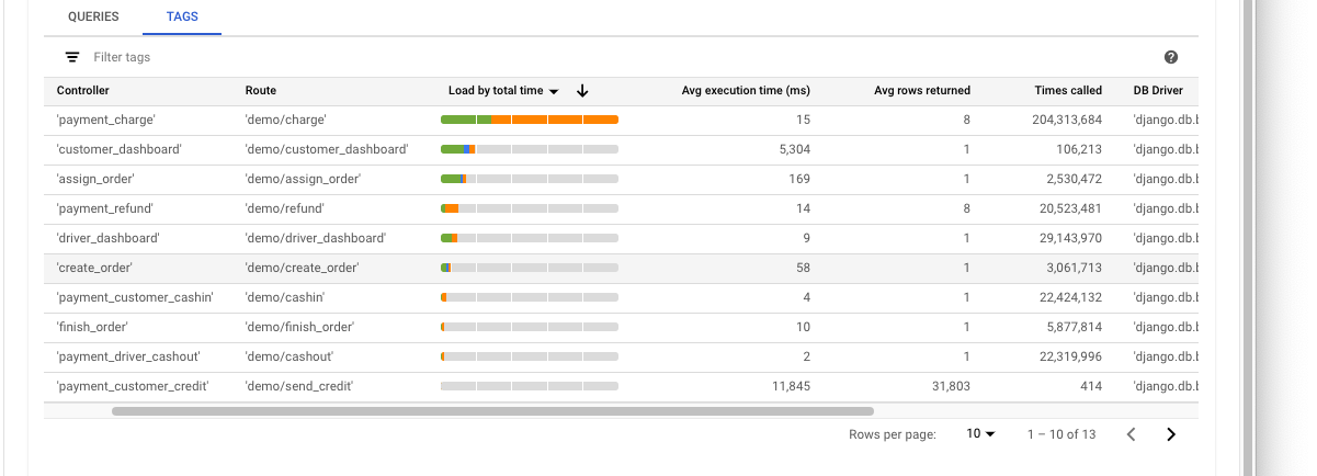
    Nimesh Bhagat, a product manager for Google, said Sqlcommenter is designed to make it simpler to correlate application and database telemetry. OpenTelemetry provides a mechanism for collecting logs, metrics and traces that is being advanced under the auspices of the Cloud Native Computing Foundation (CNCF).

    The challenge organizations using OpenTelemetry to collect that data will face is the need for tools to query that data in whatever platform it ultimately resides, noted Bhagat. OpenTelemetry previously lacked a common standard by which application tags and traces can be sent to databases and correlated with an application stack. Google envisions that IT teams will either employ Sqlcommenter to explore data or access via platforms such as Cloud SQL Insights or a third-party application performance management (APM) platform.

    Google made Sqlcommenter available as open source software earlier this year. It is designed to enable object–relational mappings (ORMs) to augment SQL statements before execution by, among other things, providing access to comments containing information about the application code that caused its execution.

    Sqlcommenter also allows OpenTelemetry trace context information to be propagated to the database, enabling correlation between application traces and database query plans that ultimately should make it easier to, for example, determine the root cause of a performance issue involving a microservices-based application making calls to a database. Sqlcommenter is primarily designed to be employed by full-stack developers that have some familiarity with how to use SQL to query data residing in an observability platform, noted Bhagat.

    Specifically, Sqlcommenter is designed to provide deeper insights into the performance of backend databases by simplifying the process of correlating slow queries with source code. It currently supports Python, Java, Node.js and Ruby languages along with ORMs such as Django, Sqlalchemy, Hibernate, Knex, Sequelize and Rails.

    As the number of applications that are instrumented using open source software continues to steadily increase, the amount of data that a DevOps team could potentially query also will steadily increase. Cloud storage platforms have made it easier to store that data at an affordable cost but the next challenge is clearly going to be finding a way to surface meaningful insights from all that data. Undoubtedly, achieving that goal will require everything from query tools to machine learning algorithms capable of identifying patterns at a level of scale that would not otherwise be possible.

    In the meantime, DevOps teams can look forward to being able to attain a level of observability that previously could only be achieved at a cost that tended to limit the number of applications organizations would instrument. At a time when the dependencies between applications increases with each passing day, that level of observability will soon prove indispensable.

  • The SolarWinds Query Report 2021: Database Priorities and Pitfalls

    The SolarWinds Query Report 2021: Database Priorities and Pitfalls

    The rise of hybrid IT and the accelerated adoption of cloud-native apps have evolved traditional database design, management and monitoring. Workloads are rapidly shifting to the cloud and application performance is heavily dependent on the performance of the underlying database. Meanwhile, the global COVID-19 pandemic has forced companies to make significant changes in the last year. Although it was and is a necessity, the transition to remote work and many organizations’ rapid pivots in strategy posed significant challenges for the technology professionals tasked with supporting new employee demands and shifting business priorities.

    As a result, organizations are increasingly acknowledging the importance of database performance management and strategy to ensure their most valuable asset: Data. SolarWinds recently revealed the findings of The SolarWinds Query Report 2021: Database Priorities and Pitfalls, which examines the current state of database management, evaluates the primary challenges database professionals face today and outlines how database professionals can best overcome these challenges.

    The North American results are based on responses to an online survey fielded in February 2021, which included participation from 331 technology professionals responsible for database performance management in the U.S. and Canada from public and private sector small, mid-size and enterprise organizations.

    Among many other key findings, this year’s report revealed the following:

    Increasing Complexity

    Database design and management are evolving in tandem with increased complexity, and IT professionals are on the verge of a significant shift in strategy that embraces cloud database-as-a-service (DBaaS) platforms as critical database performance success factors.

    • Though nearly 80% of the respondents said Microsoft SQL Server is the most critical platform in use today, there’s a relatively even split between the second, third, and fourth most-used platforms: cloud DBaaS (54%), Oracle (47%) and MySQL (43%).
    • As tech pros keep pace with advances in database platforms and indicate an intended shift toward cloud DBaaS adoption (33% of the respondents ranked cloud DBaaS as the number-one priority database platform to adopt over the next three years), the new mix of traditional/cloud DBaaS platforms will also require new skills.
    • Complexity increased in response to COVID-19 and the transition to remote work over the past year, according to 31% of respondents, who cited increased data demands from users, increased volume of data and security/compliance issues (such as GDPR) as the top three drivers of added complexity.

    The industry’s acknowledgment of cloud DBaaS platforms as critical success factors for database performance is now underway. When it comes to cloud migration (especially amidst a pandemic dramatically accelerating planning and execution of cloud computing and digital transformation), database professionals should start with a basic data and code cleanse and ensure only what’s truly needed is being migrated to reduce complexity and overall cost (we know cloud computing costs can add up). A comprehensive, successful migration strategy should also include a detailed assessment of the data estate—what dependencies or complex coding features exist? Remember, everything interconnected with a database has to go with it to the cloud, so taking these preliminary steps will help organizations avoid surprises down the road.

    Database Security/Compliance Influence Priorities

    The cloud and security/compliance are key factors influencing priorities and resource allocation in 2021 and beyond.

    • Nearly 60% of tech pros surveyed stated that of the data/systems currently managed within their organization, less than 25% are in the cloud. But this is expected to change, as 36% of respondents reported integrating cloud DBaaS is one of their organization’s top priorities in 2021.
    • Two-fifths of the respondents anticipated bigger budget allocations in 2021 (compared to 2020) for cloud services and security/compliance (42% and 39%, respectively).

    Managing database platforms is a big undertaking—a balancing act between proactive and reactive responses. But tech pros must make sure they’re covering all their bases, especially when it comes to security and compliance (and, on occasion, cost and licensing). Time and time again, we see these four big-ticket items pushed to the bottom of the priority list, and falling at one of these hurdles can do a great deal of damage. The new generation of legal compliance has real teeth if you fail to comply with the law. A simple cost-benefit analysis can be the proof point you need to highlight the potential impact of not upskilling in one of these areas and can give you a reason to move it back to the top of the priority list.

    Maintenance Constraints

    Database professionals devote more than a third of their day to database maintenance. This constrains both time and opportunity for activities such as innovation and upskilling in response to increased complexity and data-driven initiatives.

    • Maintenance work accounts for a greater portion of database professionals’ time when compared to other tasks. One-third of the tech pros surveyed stated one of the top areas where they spend the most time as a database/data/tech pro is maintenance (33%) and database development (22%).

    Daily database maintenance consumes time tech pros could otherwise be spending on things like upskilling or innovating new ways of working. For example, nearly half of those polled stated performance/query tuning was one of the top three skills/tools they believed they could develop/improve to better manage increasing database complexities, followed by security management and data engineering (45% and 41%, respectively). One of the best ways to work smarter, not harder: Mitigate downtime spent on maintenance and enable efficiency is to implement appropriate automation and monitoring tools. When implemented properly, automation and monitoring solutions can improve overall performance and eventually lead to reduced costs. Additionally, they can free up tech pros’ time, allowing them to focus on more proactive database performance management.

    The report reveals just how quickly the database architecture and operations tech pros are managing in today’s organizations are changing—and the web of management complexity accompanying this change. With application availability and performance as critical business drivers, the database has long been the linchpin of today’s IT environments. However, against the headwinds of increasingly diversified platforms and reduced resources, tech pros must be equipped to do more than reactive maintenance in environments that keep adding more databases with each passing day.

    Tech pros must capitalize on the opportunity ahead to maximize the performance potential of cloud-hosted databases and ensure the successful optimization of their organizations’ data.

  • DevOps Database Platforms Slash DX Bottlenecks

    DevOps Database Platforms Slash DX Bottlenecks

    An enterprise with many databases and various data requirements for DevOps continuous delivery presents a problem. For example, test data provisioning is a challenge today, particularly in pre-release testing of database updates. Standard practices involve shared database environments that need to be maintained from one test to the next, slowing test cycles and generally not fitting into an automated CI pipeline. As I explained in A New DevOps Database Platform is Needed, at best, it makes things chaotic; at worst, problems with database integrations with DevOps is a gross impediment to overall organization agility—which undermines the very purpose that DevOps is meant to serve.

    A recent whitepaper, A New Kind of DevOps Database Platform, indicates that there are multiple reasons why a new kind of DevOps database platform is needed, which are:

    • Compatibility requirements
    • Integration with current CI/CD pipelines
    • Integration with portfolios of value stream management
    • Infrastructure cost efficiency
    • Productivity for developers, testers and operations
    • Security and governance
    • DevOps performance

    The paper explained that a DevOps database platform requires the following capabilities to satisfy these requirements.

    • Automated database provisioning: the ability to deploy a database using automated procedures.
    • Database cloning: writable database environments are delivered on demand, based on a built versioned image.
    • Distributed repository: database images can reside on Linux and Windows servers, as well as storage systems.
    • Simple declarative builds: a simple, predefined method to make the creation of versioned data images simple, while enabling user/group access controls, data masking and other data engineering functions.
    • Scalable data cloning: database clones are served on demand, with many simultaneous clones served from a single image.
    • Comprehensive database support: the repo supports all common relational, NoSQL, machine learning and file-based data stores.
    • Versioned databases: each image becomes a versioned, immutable DevOps artifact.
    • Deploys equally to all cloud environments: DevOps databases can be deployed and operated on any on-premises infrastructure or cloud.
    • Cross-platform:  DevOps databases can be deployed and operated on common operating system environments such as Windows and Linux.
    • Security features including access management, data masking and encryption: database images easily incorporate access control, data masking and synthetic test data via SQL scripts, batch files or command line tools.
    • Compatible with CI/CD platforms:  DevOps databases can be deployed and operated equally well in multiple CI/CD platform tools such as Azure DevOps, Jenkins and CloudBees.
    • Compatible with containers and container orchestrators: DevOps databases can be deployed and operated equally well in multiple container environments such as Docker, Kubernetes and Red Hat OpenShift.
    • Deliver writeable data at the speed of DevOps: Deliver writable databases in seconds.
    • API for easy integration with DevOps tools: An API is available to enable integration of the DevOps database control plane with other tools.
    • Audit logging: The DevOps database includes a complete audit log of operations.

    Transforming to the New Database DevOps Platform

    A DevOps database platform in an enterprise requires more than simply buying and installing software and telling everyone to use it. With multiple entrenched database platforms already in place, there are practical and political considerations that must be overcome. Introducing any change to a large group of applications in an enterprise can be chaotic, and will often be more costly and take too much time if the changes are not compelling.

    To be sufficiently compelling, the database DevOps platform needs to be affordable, easy to understand, easy to set up and use with a wide variety of CI/CD pipelines. The following will be sufficiently compelling benefits to drive adoption:

    • Versioned, secure database environments or images managed as a DevOps artifact.
    • Images can be built and managed by the DevOps team, without requiring new infrastructure.
    • Multi-DB and multi-TB data environments in seconds.
    • Database environments can be served on demand for a CI/CD pipeline.
    • Lower-level database environment infrastructure is streamlined, with a single VM capable of supporting many simultaneous database environments which drives an immediate cost savings and positive ROI.
    • Data security and governance benefits with versioned database environments, with built-in and auditable security policies.

    What This Means

    Digital transformation is imperative for modern enterprises and organizations to remain competitive. However, the transformations of many enterprises and organizations are seriously impeded by the challenges of integrating databases into their DevOps application pipelines and value streams. A new DevOps database platform can allow the databases to be treated like any other DevOps artifacts that are orchestrated and automated within the DevOps toolchains.

    Suggested resources for automating database environment delivery include Windocks, Cohesity and other storage appliances that provide virtualized (cloned) database environments that can be adapted for DevOps purposes. I want to particularly acknowledge input from Windocks, who has introduced a DevOps data repo that features database virtualization on standard Linux and Windows servers, for versioned data environments and CI pipelines and cloud-native support for data delivery for containers, Kubernetes and conventional instances.

  • Hasura Extends Scope of GraphQL API Platform

    Hasura Extends Scope of GraphQL API Platform

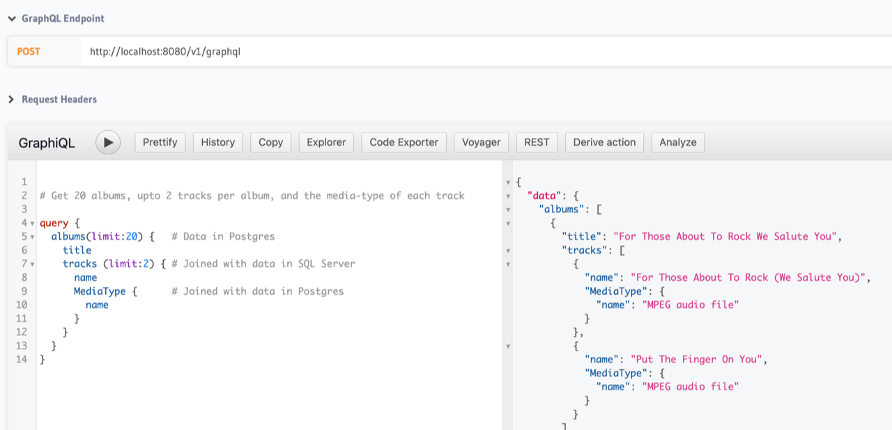
    During its online an HasuraCon ’21 conference, Hasura today announced that it has made it possible for developers to employ GraphQL application programming interface (APIs) to launch queries against data residing in multiple databases.

    At the same time, Hasura announced a preview of schema sharing capabilities along with support for workflows based on GitOps processes that it will make generally available later this year. The Hasura Cloud platform can now deploy local migrations from staging to production with a simple git push in addition to accessing previews of applications on every pull request to the git repository.

    The schema sharing capability added to the Hasura GraphQL Engine is intended to bridge the gap between beginner and power users by allowing them to share and install samples of permissions, relationships and metadata. In addition to improving collaboration, the goal is to make it easier to onboard software engineers as projects evolve and become more complex.

    Originally developed by Facebook, GraphQL has emerged as a popular alternative to REST APIs because it enables developers to retrieve data at a more granular level, which results in improved performance.

    Hasura is a provider of an instance of a GraphQL engine the company has developed around a project that is now hosted by the GraphQL Foundation, an arm of the Linux Foundation. The GraphQL Foundation counts among its members Airbnb, Amazon Web Services (AWS), Apollo, Coursera, Elementl, Facebook, GitHub, IBM, Intuit Hasura, Paypal, Prisma, Shopify and Twitter.

    GraphQL provides a complete description of the data made available via an API and is organized in terms of types and fields rather than traditional endpoints. In addition to clarifying what data is available via that API, developers can employ types to avoid writing manual parsing code.

    Since last summer, Hasura has been making available a pilot of a GraphQL implementation that is capable of supporting remote joins across disparate databases. That capability is critical because data sets that are related to a specific business process may wind up being stored in multiple databases.

    Hasura

    Tanmai Gopal, Hasura CEO, said the open source Hasura GraphQL Engine has already been downloaded more than 250 million times this year. Downloads in 2020 reached 100 million. The challenge is that while GraphQL offers a superior alternative to REST APIs, most of the API tooling that exists within organizations is still designed around REST APIs, noted Gopal.

    To accommodate that reality, Hasura has made a tool available that will convert a query designed using GraphQL into a set of calls that are compatible with REST APIs. Developers still gain the benefits of being able to launch more granular queries, noted Gopal.

    REST APIs, in general, are becoming more problematic as organizations embrace microservices-based applications. It often takes minutes to refresh a simple dashboard because of the amount of data that REST APIs are trying to pull from various data sources. As organizations embrace digital business transformation, they are also encountering application latency issues that can be traced back to the amount of data being called from multiple microservices.

    Hasura says in addition to providing a more efficient method to access data, Hasura is also working on adding caching capabilities to its core engine to further improve performance.

    It’s not clear at what rate GraphQL might replace REST APIs, but DevOps teams should assume organizations will wind up employing a mix of both for years to come. The challenge is going to be determining when to make the transition as organizations become more dependent on APIs.

  • No-Nonsense Guide to Distributed Databases

    No-Nonsense Guide to Distributed Databases

    I got my first DBA job 15 years ago, and quite a few things have changed since then. The amount of data exploded, we saw the rise of NoSQL, and business logic moved away from being stored in relational databases to applications.

    To this day, the three pillars of reliability, scalability, and maintainability are the banes of a DBA’s existence. To spice things up, your monthly cloud bill for managed databases just made your CTO lose the will to live.

    So, now you have two extra things to worry about in addition to these three pillars: cost efficiency and vendor-agnosticism.

    In this article, I’ll (try to) run an open source, new-generation database, benchmark it and touch on some of the challenges of being cloud-neutral.

    TL;DR

    • Solving the SQL vs. NoSQL dilemma in the Kubernetes world
    • How to leverage a distributed SQL database in a multi-cloud world
    • Taming performance – single cloud versus multi-cloud
    • Running TPC-C as a transactional benchmark
    • Taming the costs – the question of egress costs

    New Packaging For a New Age

    Just five years ago, people were like, “Containerizing stateless microservices? Sure! No problem.”

    But when you actually containerize a database, your persistence layer is asking for trouble.

    Over time, containers grew on us. Now, it’s the default way of packaging and shipping software. Heck, even AWS Lambda caved and started running container images. Databases just couldn’t resist.

    Once a database is containerized – say, a PostgreSQL database – Kubernetes takes over dealing with some of the more painful aspects of reliability and maintainability (with the help of middleware-specific operators).

    Containers decouple data from the runtime, so upgrades and configuration are easier through infrastructure-as-code (YAML). Hardware failure and maintenance windows are covered by Kubernetes’ built-in capability to reschedule pending pods on surviving nodes. Full scheduled backups or point-in-time recovery are in the hands of the operator’s automation.

    But what about scalability?

    Kubernetes’ vertical pod autoscaler can adjust container resources, deleting and recreating pods with new resource settings. As a traditional relational database, PostgreSQL can have only one primary replica that writes data. This means that you’ll be facing a  short downtime while the new pod comes online. The majority of workloads are about five times oversized, so while sizing is painful, it’s better than no sizing at all (please, have mercy on your CTO’s budget).

    NoSQL has none of these limitations. Databases like Cassandra were built for scaling horizontally without downtime.

    Enter Distributed SQL

    What if we could blend Google Spanner’s ability to operate at distances with strong ACID consistency, Cassandra’s scaling and PostgreSQL compatibility?

    This is where YugabyteDB helps.

    YugabyteDB is an open source, relational, distributed SQL database management system. It was designed to handle large amounts of data across multiple availability zones and geographic regions, all the while delivering single-digit latency, high availability and no single point of failure.

    I hate when the new kid on the block brings their own syntax language because, you know, their case is so very special – just like everybody else’s.

    Yugabyte doesn’t do that. They have a wicked-smart storage layer (inspired by Google Spanner) that reuses the PostgreSQL query engine. This means no mental strain on the development team – you get to use the time-tested, marketable and incredibly powerful PostgreSQL language-level features that many are already comfortable with.

    If Google Spanner is so inspiring, why is it not taking over the world of distributed SQL? Well, it’s available only as SaaS, and heavily depends on the specifics of Google Cloud hardware like atomic clocks (trueTime) and Google’s backbone network. If your private data center or favorite cloud provider is not GCP – well, no Spanner for you, my friend. Personally, I’d be hesitant to marry into the ultimate vendor lock-in. Yugabyte doesn’t have any dependencies and would happily run on any cloud, private data center, VM or bare metal – and if your coffee machine runs Docker containers, you can run Yugabyte there, as well.

    If Yugabyte is robust, scalable and easily maintainable, you have the top three pillars covered. But what about the other two pillars your CTO is nagging you about (cost efficiency and a vendor-agnostic approach)?

    How to Make Your Database Vendor-Agnostic

    Being vendor-agnostic means being able to switch between major cloud providers at any point without depending on prohibitively expensive services like DynamoDB. This approach also allows you to leverage inefficiencies in cloud pricing so you can look for new opportunities to reduce cost and dynamically shift resources between cloud providers online.

    This is something CAST AI can do.

    The CAST AI platform acts as a cloud abstraction and makes the whole multi-cloud, vendor-agnostic requirement quite trivial.

    Developers just interact with standard Kubernetes (no CRDs), and the complexity of several clouds is abstracted. A Kubernetes cluster in CAST AI can span across several cloud providers at the same time, bringing some unique cost optimization opportunities.

    What if spot/preemptible instance interruption wasn’t totally random anymore, but something you could actually predict? You could be proactive and—by operating in several compute bidding markets at the same time—reduce the risk of running out of capacity.

    Why not slash your monthly cloud bill radically by running some of the database containers on spot/preemptible nodes?

    Highly Available Stateful Application on Multi-Cloud

    Yugabyte on a multi-cloud CAST AI Kubernetes cluster is a robust design without a single point of failure.

    Active/Passive solutions are so ’90s—failovers cause brief downtime, and DBAs tend to leave the failover to be manually initiated due to occasional short-lived network blips. Active/Passive solutions constantly require testing and validation. Will your disaster recovery work on darker days? Because these tests cause downtime, nobody does them regularly.

    The best highly available solutions are active-active, don’t require user failover, and don’t rot if not tested regularly.

    CAST AI has a tutorial in place that takes you through every step of building the above solution in about 10 minutes, from scratch.

    Go ahead, open your cloud provider’s console and release your inner chaos monkey by killing Yugabyte, business app pods or whole Kubernetes nodes.

    CAST AI, Yugabyte, and Kubernetes were built with a core tenet that nothing is guaranteed; nothing should be shared. But keep in mind, consensus algorithms work when there’s still a majority left to vote N/2 + 1.

    You may be asking, what’s the performance impact of increasing resiliency when going multi-cloud with a distributed database?

    Let’s find out.

    Let’s benchmark a distributed Yugabyte database on top of CAST AI Kubernetes spanning AWS and GCP. These cloud providers are arbitrary choices here; Azure or DigitalOcean can be used in the mix, as well. We picked GCP and AWS because their VMs boot up a bit faster.

    Mono-Cloud Vs. Dual-Cloud Network Benchmark Results

    Let’s compare a Yugabyte containerized database on Kubernetes in a single-cloud scenario versus a distributed database working in two different clouds.

    Setup

    We took the OSS Yugabyte HELM chart with the image version “2.5.1.0” with the replication factor of 3.

    Role

    YB-Master

    YB-Tserver

    Description

    Control plane, consensus

    Serves data

    CPU

    3 CPUs

    7 CPUs

    RAM

    3 GiB

    14 GiB

    Storage

    50 GiB

    300 GiB

    Remote Network Block storage:

    • EBS gp2 (300 IOPs)
    • Standard persistent disk (R225/W450 IOps)

    Nine pods, each on a separate VM to ensure plenty of resources:

    Mono Cloud

    Regional GKE k8s cluster with 9x GCE N2d-standard-8 distributed in three availability zones. Casual VPC network in Google’s US-East4 region.

    Dual Cloud

    AWS EC2 3x c5a.2xlarge

    GCP GCE 6x n2d-standard-8

    A network between cloud providers set up with a Wireguard-based full mesh VPN that encrypts traffic end-to-end (also inside the same VPC).

    To minimize noise from compute and local storage efficiency, we didn’t optimize for cost but wanted to isolate and better understand how distributed databases would work in situations where database nodes are distributed single-digit milliseconds away (in this example, less than 9 ms).

    Nine milliseconds of network round trip latency means a lot of flexibility in choosing between data center providers distributed within a few hundred miles.

    The majority of cloud provider regions lack imagination and are clustered in the geographic vicinity of a densely populated metropolis. California, northern Virginia, Montreal, São Paulo, London, Frankfurt, Amsterdam, Mumbai, Tokyo, Singapore, Sydney, etc.

    So, what are your options in, say, Frankfurt? AWS, Azure, GCP, DigitalOcean, Oracle, Alibaba, IBM Cloud, Hetzner, Linode—not to mention the white-label providers.

    We carried out tests on U.S. East (Ashburn) and Europe Central (Frankfurt) with similar results.

    How We Measured It

    If we want to test relational database performance – the gold standard ruler to date is a synthetic TPC-C benchmark.

    Why did we choose that? Because it’s the most mature OLTP benchmarking test suite that has stood the test of time. As stated here:

    “While the benchmark portrays the activity of a wholesale supplier, TPC-C is not limited to the activity of any particular business segment, but, rather represents any industry that must manage, sell, or distribute a product or service.”

    We loaded an identical Yugabyte configuration in both scenarios with 300 warehouses worth of data and then ran benchmarks several times.

    Each test took half an hour, and the output was the single most important metric: transactions per minute. The test also provided different outputs per type of transaction, average and 99th percentile duration in milliseconds.

    Results

    This table shows a comparison of TPC-C results with the average duration for a single cloud on Google and AWS + Google in the same region, US-East.

    300 warehouses

    Mono Cloud

    Dual Cloud

    Num New Order transactions per 1800 s

    113,071

    113,247

    TPM-C

    3,769

    3,774

    Efficiency

    97.6%

    97.8%

    NewOrder Latency avg msec

    580.2

    498.8

    Payment Latency avg msec

    30.8

    46.7

    OrderStatus Latency avg msec

    33.8

    32.4

    Delivery Latency avg msec

    123.1

    174.9

    StockLevel Latency avg msec

    239.4

    465

    And comparing the 99th percentile:

    300 warehouses

    Mono Cloud

    Dual Cloud

    NewOrder Latency  p99 msec

    6985.6

    5498.7

    Payment Latency p99 msec

    110.5

    157.5

    OrderStatus Latency p99 msec

    146.3

    185.1

    Delivery Latency p99 msec

    331.5

    696.8

    StockLevel Latency p99 msec

    712.3

    1083.3

    As you can see, the difference between the mono cloud and dual cloud scenarios is quite small.

    Some operations, like OrderStatus, are plain read operations. The nearest server can quickly respond with data to the client—usually, a microservice running on the same K8s cluster.

    Yugabyte’s lowest isolation level is a snapshot. This means that those reads are protected from the undesirable effect of the “dirty read.”

    What about writes?

    Writes are a bit more expensive. Raft consensus, hybrid logical clocks and lockless multi-version concurrency control (MVCC) algorithm magic—all of this means a lot more chatter and replication between nodes to get write committed.

    We see that, in payment and delivery operations duration (30ms vs. 46ms and 123ms vs. 174ms, respectively) the geographic distances start to be noticeable.

    The actual network latency between nodes in different availability zones in the mono cloud scenario without network overlay and encryption is, on average, about 0.6ms. Network latency between two clouds with overlay (VXLAN) and encryption (Wireguard) is about 5ms.

    The laws of physics aren’t going away anytime soon. But as we can see, the results are much better than expected.

    YMMV, but industry accepted norm is that the majority of IO operations will be reads, at 70%; only remaining 30% writes, reducing the impact of speed of light even further.

    Having said that, the gold standard for measuring OLTP database performance for the last two decades says that performance results are identical (TPM-C 3’769 vs. 3’774).

    Data Gravity and Egress Costs

    Data gravity refers to a scenario where compute gravitates closer to data.

    For example, if you have a hybrid cloud or multi-cloud strategy but your data stays in a single location like an on-premises data center. Most of the compute with stateless services will tend to stay in the same data center, closer to data.

    The whole point of multi-cloud and a high-performing distributed database was to get rid of data gravity. If we have the same data on two or more clouds, then the data gravity effect disappears.

    If all your data is replicated to several locations, what about network traffic costs?

    All cloud providers allow unlimited incoming (ingress) data. It doesn’t matter where data is coming from—if it’s your on-premises data center, a different cloud provider, the dark web or most cloud-native services. All the incoming data is free.

    “You can bring as much data as you want to us. But if you want to take your data back – sorry, you need to pay.” This is universal between all cloud providers. All the outgoing (egress) traffic from your availability zone is paid! Some cloud providers, like Oracle Cloud, are very generous with egress costs, and companies like Zoom saved a ton of money when they moved some of Zoom’s infrastructure to Oracle Cloud.

    DigitalOcean gives a generous egress monthly allowance per Droplet (VM), depending on size and how long you run it. But, at a minimum, it starts at Terabyte per smallest Droplet. The monthly egress allowance is aggregated in your account, and you pay only for the combined extra.

    All clouds have some minimal free tier—but in general, egress costs start at around 10 cents per GB of data sent outside VPC, and, on average, 2 cents for data between availability zones in the same VPC (I bet you didn’t know that you pay 1cnt/GB in AWS and Azure for incoming traffic coming from same VPC/Vnet from another AZ).

    If you send more traffic, your cost per GB falls. The first drop is at 10TB and generally flattens at around 5 cents at ~150TB.

    How does it make you feel when cloud providers charge an eye-watering 97% margin on that egress traffic? It’s like we’re back in 1995 with dial-up modems, right?

    There is a more cost-effective alternative. But first, let’s answer the ‘Will it Blend?’ question. Let’s add Direct Connect, Express Route, Cloud Interconnect and Layer 2 or Layer 3 providers like Equinix or Megaport. Yes, you get a Dedicated Fiber Link smoothie out of the blender.

    Dedicated fiber link slashes costs to a mere 2 cents per GB. And if you have more egress traffic than 7TB, it’s more cost-effective than relying on the weird discount models from cloud providers.

    You might be thinking, “2 cents for every GB?! That’s way too much! I’m using RDS—yes, I have vendor lock-in and data gravity—but at least I have none of the problems with egress cost, resilience, scalability and overall affordability of the service, right?”

    That’s just the result of an opaque billing design.

    https://twitter.com/QuinnyPig/status/1372598432095891458

    All the traffic between Availability Zones in all clouds is paid at 2 cents per GB of egress+ingress. The only place where you pay for ingress is between Availability Zones in the same region (AWS/Azure). Some managed services offer free replication, but they charge double on compute costs, etc.

    Through the ServiceTopology feature, Kubernetes can keep your application pod’s traffic inside the same cloud service provider Availability Zone and cloud, to avoid round robin, random calls between clouds. This means that you get the best latency and pay no traffic premium.

    Most of the database activity is reads (70/30, YMMV) and are effectively free, egress-wise (coming from the local AZ due to the Kubernetes topology awareness). So, the only thing you replicate and subject to egress costs is your database change delta rate per month.

    Now you can see that the issue of egress costs is an incredibly overstated problem.

    The overwhelming push to the public cloud over the last decade brought on new challenges like vendor lock-in, data gravity and eye-watering monthly infrastructure bills.

    During that time, innovation in non-traditional RDBMS, containerization and workload scheduling removed some of the old barriers.

    Running a hands-free, strongly consistent, highly available and scalable database in heterogeneous data centers on a budget was a monumental task a decade ago. Today, it has become an affordable best practice for running our business applications.